Page 113 - Applied Statistics Using SPSS, STATISTICA, MATLAB and R

92 3 Estimating Data Parameters

In parameter estimation one often needs to use percentiles of random
distributions. We have seen that before, concerning the application of percentiles
of the normal and the Student’s t distribution. Later on we will need to apply
percentiles of the chi-square and F distributions. Statistical software usually
provides a large panoply of probabilistic functions (density and cumulative
distribution functions, quantile functions and random number generators with
particular distributions). In Commands 3.3 we present some of the possibilities.
Appendix D also provides tables of the most usual distributions.

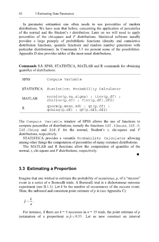
Commands 3.3. SPSS, STATISTICA, MATLAB and R commands for obtaining
quantiles of distributions.

SPSS Compute Variable

STATISTICA Statistics; Probability Calculator

MATLAB norminv(p,mu,sigma) ; tinv(p,df) ;
chi2inv(p,df) ; finv(p,df1,df2)
R qnorm(p,mean,sd) ; qt(p,df) ;
qchisq(p,df) ; qf(p,df1,df2)

The Compute Variable window of SPSS allows the use of functions to
compute percentiles of distributions, namely the functions Idf.IGauss , Idf.T ,
Idf.Chisq and Idf.F for the normal, Student’s t, chi-square and F
distributions, respectively.
STATISTICA provides a versatile Probability Calculator allowing
among other things the computation of percentiles of many common distributions.
The MATLAB and R functions allow the computation of quantiles of the
normal, t, chi-square and F distributions, respectively.

3.3 Estimating a Proportion

Imagine that one wished to estimate the probability of occurrence, p, of a “success”
event in a series of n Bernoulli trials. A Bernoulli trial is a dichotomous outcome
experiment (see B.1.1). Let k be the number of occurrences of the success event.
Then, the unbiased and consistent point estimate of p is (see Appendix C):

k
ˆ
p = .
n

For instance, if there are k = 5 successes in n = 15 trials, the point estimate of p
(estimation of a proportion) is ˆ =p . 0 33 . Let us now construct an interval