Page 114 - Applied Statistics Using SPSS, STATISTICA, MATLAB and R

3.3 Estimating a Proportion 93

estimation for p. Remember that the sampling distribution of the number of
“successes” is the binomial distribution (see B.1.5). Given the discreteness of the
binomial distribution, it may be impossible to find an interval which has exactly
the desired confidence level. It is possible, however, to choose an interval which
covers p with probability at least 1– α.

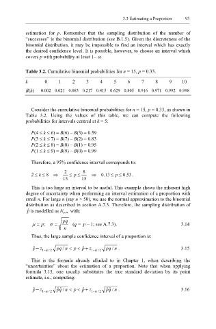
Table 3.2. Cumulative binomial probabilities for n = 15, p = 0.33.

k 0 1 2 3 4 5 6 7 8 9 10
B(k) 0.002 0.021 0.083 0.217 0.415 0.629 0.805 0.916 0.971 0.992 0.998

Consider the cumulative binomial probabilities for n = 15, p = 0.33, as shown in
Table 3.2. Using the values of this table, we can compute the following
probabilities for intervals centred at k = 5:

P(4 ≤ k ≤ 6) = B(6) – B(3) = 0.59
P(3 ≤ k ≤ 7) = B(7) – B(2) = 0.83
P(2 ≤ k ≤ 8) = B(8) – B(1) = 0.95
P(1 ≤ k ≤ 9) = B(9) – B(0) = 0.99

Therefore, a 95% confidence interval corresponds to:

2 8
2 ≤ k ≤ 8 ⇒ ≤ p ≤ ⇒ . 0 13 ≤ p ≤ . 0 53.
15 15
This is too large an interval to be useful. This example shows the inherent high
degree of uncertainty when performing an interval estimation of a proportion with
small n. For large n (say n > 50), we use the normal approximation to the binomial
distribution as described in section A.7.3. Therefore, the sampling distribution of
p ˆ is modelled as N µ,σ with:
pq
µ = p; σ = (q = p – 1; see A.7.3). 3.14
n
Thus, the large sample confidence interval of a proportion is:

p ˆ − z 1 α 2 / pq n / < p < p ˆ + z 1 α 2 / pq n / . 3.15
−
−

This is the formula already alluded to in Chapter 1, when describing the
“uncertainties” about the estimation of a proportion. Note that when applying
formula 3.15, one usually substitutes the true standard deviation by its point
estimate, i.e., computing:

p ˆ − z 1 α 2 / q p n / ˆ ˆ < p < p ˆ + z 1 α 2 / q p n / ˆ ˆ . 3.16
−
−