Page 116 - Applied Statistics Using SPSS, STATISTICA, MATLAB and R

3.4 Estimating a Variance 95

is to convert the variable being analysed into a Bernoulli type variable, i.e., a
binary variable with 1 coding the “success” event, and 0 the “failure” event. As a
matter of fact, a dataset x 1, …, x n, with k successes, represented as a sequence of
values of Bernoulli random variables (therefore, with k ones and n – k zeros), has
the following sample mean and sample variance:

x = ∑ n = i 1 x i n / = k / n ≡ p. ˆ

∑ n x ( i − p) ˆ 2 p nˆ − 2 p kˆ + k n
2
2
v = i 1= = = p ˆ ( − p ) ≈ p q ˆ ˆ .
ˆ
−
−
−
n 1 n 1 n 1

In Example 3.5, variable DISPL with values 1 for “Yes” and 2 for “No” is
converted into a Bernoulli type variable, DISPLB, e.g. by using the formula
DISPLB = 2 – DISPL. Now, the “success” event (“Yes”) is coded 1, and the
complement is coded 0. In SPSS and STATISTICA we can also use “if” constructs
to build the Bernoulli variables. This is especially useful if one wants to create
Bernoulli variables from continuous type variables. SPSS and STATISTICA also
have a Rank command that can be useful for the purpose of creating Bernoulli
variables.

Commands 3.4. MATLAB and R commands for obtaining confidence intervals of
proportions.

MATLAB ciprop(n0,n1,alpha)

R ciprop(n0,n1,alpha)

There are no specific functions to compute confidence intervals of proportions in
MATLAB and R. However, we provide for MATLAB and R the function
ciprop(n0,n1,alpha) for that purpose (see Appendix F). For Example 3.5
we obtain in R:
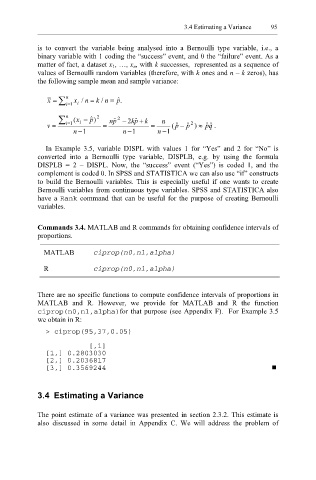
> ciprop(95,37,0.05)

[,1]
[1,] 0.2803030
[2,] 0.2036817
[3,] 0.3569244

3.4 Estimating a Variance

The point estimate of a variance was presented in section 2.3.2. This estimate is
also discussed in some detail in Appendix C. We will address the problem of