Page 111 - Applied Statistics Using SPSS, STATISTICA, MATLAB and R

90 3 Estimating Data Parameters

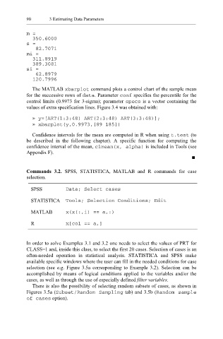
m =
350.6000
s =
82.7071
mi =
311.8919
389.3081
si =
62.8979
120.7996

The MATLAB xbarplot command plots a control chart of the sample mean
for the successive rows of data . Parameter conf specifies the percentile for the
control limits (0.9973 for 3-sigma); parameter specs is a vector containing the
values of extra specification lines. Figure 3.4 was obtained with:

» y=[ART(1:3:48) ART(2:3:48) ART(3:3:48)];
» xbarplot(y,0.9973,[89 185])

Confidence intervals for the mean are computed in R when using t.t est (to
be described in the following chapter). A specific function for computing the
confidence interval of the mean, cimean(x, alpha) is included in Tools (see
Appendix F).

Commands 3.2. SPSS, STATISTICA, MATLAB and R commands for case
selection.

SPSS Data; Select cases

STATISTICA Tools; Selection Conditions; Edit
MATLAB x(x(:,i) == a,:)

R x[col == a,]

In order to solve Examples 3.1 and 3.2 one needs to select the values of PRT for
CLASS=1 and, inside this class, to select the first 20 cases. Selection of cases is an
often-needed operation in statistical analysis. STATISTICA and SPSS make
available specific windows where the user can fill in the needed conditions for case
selection (see e.g. Figure 3.5a corresponding to Example 3.2). Selection can be
accomplished by means of logical conditions applied to the variables and/or the
cases, as well as through the use of especially defined filter variables.
There is also the possibility of selecting random subsets of cases, as shown in
Figures 3.5a (Subset/Random Sampling tab) and 3.5b (Random sample
of cases option).