Page 119 - Applied Statistics Using SPSS, STATISTICA, MATLAB and R

98 3 Estimating Data Parameters

Example 3.8
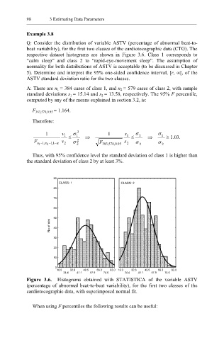
Q: Consider the distribution of variable ASTV (percentage of abnormal beat-to-
beat variability), for the first two classes of the cardiotocographic data (CTG). The
respective dataset histograms are shown in Figure 3.6. Class 1 corresponds to
“calm sleep” and class 2 to “rapid-eye-movement sleep”. The assumption of
normality for both distributions of ASTV is acceptable (to be discussed in Chapter
5). Determine and interpret the 95% one-sided confidence interval, [r, ∞[, of the
ASTV standard deviation ratio for the two classes.

A: There are n 1 = 384 cases of class 1, and n 2 = 579 cases of class 2, with sample
standard deviations s 1 = 15.14 and s 2 = 13.58, respectively. The 95% F percentile,
computed by any of the means explained in section 3.2, is:

F 383,578,0.95 = 1.164.

Therefore:

1 v 1 ≤ σ 1 2 ⇒ 1 s 1 ≤ σ 1 ⇒ σ 1 ≥ 1.03.
F 1 n − ,1 2 n − 1,1 −α v 2 σ 2 2 F 383 , 578 . 0 , 95 s 2 σ 2 σ 2

Thus, with 95% confidence level the standard deviation of class 1 is higher than
the standard deviation of class 2 by at least 3%.

90
CLASS: 1 CLASS: 2
80
70

60
50
No of obs 40

30
20

10
0
16.0 32.8 49.5 66.3 83.0 16.0 32.8 49.5 66.3 83.0
24.4 41.1 57.9 74.6 24.4 41.1 57.9 74.6

Figure 3.6. Histograms obtained with STATISTICA of the variable ASTV
(percentage of abnormal beat-to-beat variability), for the first two classes of the
cardiotocographic data, with superimposed normal fit.

When using F percentiles the following results can be useful: