Page 121 - Applied Statistics Using SPSS, STATISTICA, MATLAB and R

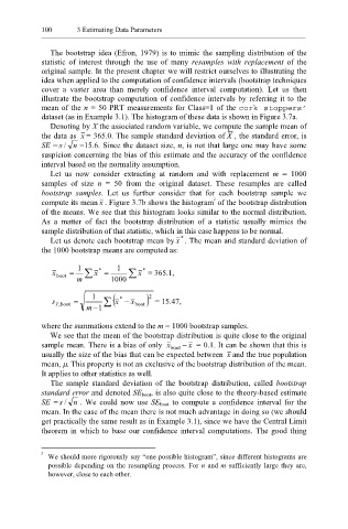
100 3 Estimating Data Parameters

The bootstrap idea (Efron, 1979) is to mimic the sampling distribution of the
statistic of interest through the use of many resamples with replacement of the
original sample. In the present chapter we will restrict ourselves to illustrating the
idea when applied to the computation of confidence intervals (bootstrap techniques
cover a vaster area than merely confidence interval computation). Let us then
illustrate the bootstrap computation of confidence intervals by referring it to the
mean of the n = 50 PRT measurements for Class=1 of the cork stoppers’
dataset (as in Example 3.1). The histogram of these data is shown in Figure 3.7a.
Denoting by X the associated random variable, we compute the sample mean of
the data as x = 365.0. The sample standard deviation of X , the standard error, is
SE = s / n =15.6. Since the dataset size, n, is not that large one may have some
suspicion concerning the bias of this estimate and the accuracy of the confidence
interval based on the normality assumption.
Let us now consider extracting at random and with replacement m = 1000
samples of size n = 50 from the original dataset. These resamples are called
bootstrap samples. Let us further consider that for each bootstrap sample we
2
compute its mean x . Figure 3.7b shows the histogram of the bootstrap distribution
of the means. We see that this histogram looks similar to the normal distribution.
As a matter of fact the bootstrap distribution of a statistic usually mimics the
sample distribution of that statistic, which in this case happens to be normal.
*
Let us denote each bootstrap mean by x . The mean and standard deviation of
the 1000 bootstrap means are computed as:

1 1
*
x boot = ∑ x * = ∑ x = 365.1,
m 1000
1 ( 2
s , x boot = ∑ * − x boot )x = 15.47,
m −1

where the summations extend to the m = 1000 bootstrap samples.
We see that the mean of the bootstrap distribution is quite close to the original
sample mean. There is a bias of only x boot − x = 0.1. It can be shown that this is
usually the size of the bias that can be expected between x and the true population
mean, µ. This property is not an exclusive of the bootstrap distribution of the mean.
It applies to other statistics as well.
The sample standard deviation of the bootstrap distribution, called bootstrap
standard error and denoted SE boot, is also quite close to the theory-based estimate
SE = s / n . We could now use SE boot to compute a confidence interval for the
mean. In the case of the mean there is not much advantage in doing so (we should
get practically the same result as in Example 3.1), since we have the Central Limit
theorem in which to base our confidence interval computations. The good thing

2
We should more rigorously say “one possible histogram”, since different histograms are
possible depending on the resampling process. For n and m sufficiently large they are,
however, close to each other.