Page 126 - Applied Statistics Using SPSS, STATISTICA, MATLAB and R

3.6 Bootstrap Estimation 105

In the above Example 3.11 we observe in Figure 3.12 a histogram that doesn’t
look to be well approximated by the normal distribution. As a matter of fact any
goodness of fit test described in section 5.1 will reject the normality hypothesis.
This is a common difficulty when estimating bootstrap confidence intervals for the
median. An explanation of the causes of this difficulty can be found e.g. in
(Hesterberg T et al., 2003). This difficulty is even more severe when the data size n
is small (see Exercise 3.20). Nevertheless, for data sizes larger then 100 cases, say,
and for a large number of resamples, one can still rely on bootstrap estimates of the
median as in Example 3.11.

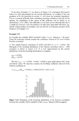
Example 3.12
Q: Consider the variables Al2O3 and K2O of the Clays’ dataset (n = 94 cases).
Using the bootstrap method compute the confidence interval at 5% level of their
Pearson correlation.
A: The sample Pearson correlation of Al2O3 and K2O is r ≡ w = 0.6922. The
histogram of the bootstrap distribution of the Pearson correlation with m = 1000
resamples is shown in Figure 3.13. It is well approximated by the normal
distribution. From the bootstrap distribution we compute:

w boot = 0.6950
SE boot = 0.0719

The bias w boot − w = 0.6950 – 0.6922 = 0.0028 is quite small (about 0.4% of the
correlation value). We therefore compute the bootstrap confidence interval of the
Pearson correlation as:

w t ± 93 . 0 , 975 SE boot = 0.6922 ± 1.9858×0.0719 = 0.69 ± 0.14

300
n
250
200

150
100

50
w*
0
0.45 0.5 0.55 0.6 0.65 0.7 0.75 0.8 0.85 0.9 0.95
Figure 3.13. Histogram of the bootstrap distribution of the Pearson correlation
between the variables Al2O3 and K2O of the Clays’ dataset (1000 resamples).