Page 127 - Applied Statistics Using SPSS, STATISTICA, MATLAB and R

106 3 Estimating Data Parameters

We draw the reader’s attention to the fact that when generating bootstrap
samples of associated variables, as in the above Example 3.12, these have to be
generated by drawing cases at random with replacement (and not the variables
individually), therefore preserving the association of the variables involved.

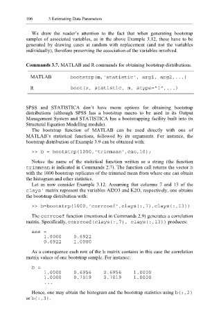
Commands 3.7. MATLAB and R commands for obtaining bootstrap distributions.
MATLAB bootstrp(m,’statistic’, arg1, arg2,...)

R boot(x, statistic, m, stype=“i”,...)

SPSS and STATISTICA don’t have menu options for obtaining bootstrap
distributions (although SPSS has a bootstrap macro to be used in its Output
Management System and STATISTICA has a bootstrapping facility built into its
Structural Equation Modelling module).
The bootstrap function of MATLAB can be used directly with one of
MATLAB’s statistical functions, followed by its arguments. For instance, the
bootstrap distribution of Example 3.9 can be obtained with:

>> b = bootstrp(1000,’trimmean’,cao,10);

Notice the name of the statistical function written as a string (the function
trimmean is indicated in Commands 2.7). The function call returns the vector b
with the 1000 bootstrap replicates of the trimmed mean from where one can obtain
the histogram and other statistics.
Let us now consider Example 3.12. Assuming that columns 7 and 13 of the
clays’ matrix represent the variables Al2O3 and K2O, respectively, one obtains
the bootstrap distribution with:

>> b=bootstrp(1000,’corrcoef’,clays(:,7),clays(:,13))

The corrcoe f function (mentioned in Commands 2.9) generates a correlation
matrix. Specifically, corrcoef(clays(:,7), clays(:,13)) produces:

ans =
1.0000 0.6922
0.6922 1.0000

As a consequence each row of the b matrix contains in this case the correlation
matrix values of one bootstrap sample. For instance:

b =
1.0000 0.6956 0.6956 1.0000
1.0000 0.7019 0.7019 1.0000
...

Hence, one may obtain the histogram and the bootstrap statistics using b( :,2)
or b(:,3) .