Page 123 - Applied Statistics Using SPSS, STATISTICA, MATLAB and R

102 3 Estimating Data Parameters

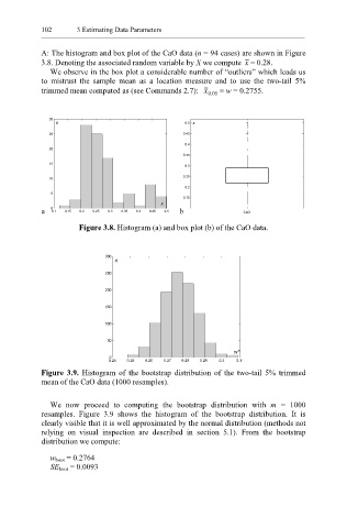
A: The histogram and box plot of the CaO data (n = 94 cases) are shown in Figure
3.8. Denoting the associated random variable by X we compute x = 0.28.
We observe in the box plot a considerable number of “outliers” which leads us
to mistrust the sample mean as a location measure and to use the two-tail 5%
trimmed mean computed as (see Commands 2.7): x . 0 05 ≡ w = 0.2755.

30
n 0.5 x
25 0.45
0.4
20
0.35
15
0.3
0.25
10
0.2
5
0.15
x
a 0 0.1 0.15 0.2 0.25 0.3 0.35 0.4 0.45 0.5 b CaO
Figure 3.8. Histogram (a) and box plot (b) of the CaO data.

300
n
250
200

150

100
50
w*
0
0.24 0.25 0.26 0.27 0.28 0.29 0.3 0.31
Figure 3.9. Histogram of the bootstrap distribution of the two-tail 5% trimmed
mean of the CaO data (1000 resamples).

We now proceed to computing the bootstrap distribution with m = 1000
resamples. Figure 3.9 shows the histogram of the bootstrap distribution. It is
clearly visible that it is well approximated by the normal distribution (methods not
relying on visual inspection are described in section 5.1). From the bootstrap
distribution we compute:

w boot = 0.2764
SE boot = 0.0093