Page 122 - Applied Statistics Using SPSS, STATISTICA, MATLAB and R

3.6 Bootstrap Estimation 101

about the bootstrap technique is that it also often works for other statistics for
which no theory on sampling distribution is available. As a matter of fact, the
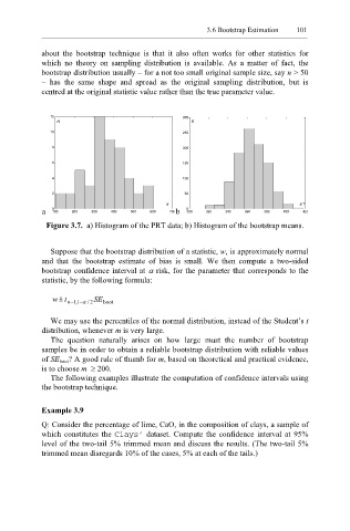
bootstrap distribution usually – for a not too small original sample size, say n > 50
− has the same shape and spread as the original sampling distribution, but is
centred at the original statistic value rather than the true parameter value.

12 300
n n
10 250

8 200
6 150

4 100
2 50
x x *
a 0 100 200 300 400 500 600 700 b 0 300 320 340 360 380 400 420
Figure 3.7. a) Histogram of the PRT data; b) Histogram of the bootstrap means.

Suppose that the bootstrap distribution of a statistic, w, is approximately normal
and that the bootstrap estimate of bias is small. We then compute a two-sided
bootstrap confidence interval at α risk, for the parameter that corresponds to the
statistic, by the following formula:

w t ± n− 1 , 1 − α 2 / SE boot

We may use the percentiles of the normal distribution, instead of the Student’s t
distribution, whenever m is very large.
The question naturally arises on how large must the number of bootstrap
samples be in order to obtain a reliable bootstrap distribution with reliable values
of SE boot ? A good rule of thumb for m, based on theoretical and practical evidence,
is to choose m ≥ 200.
The following examples illustrate the computation of confidence intervals using
the bootstrap technique.

Example 3.9
Q: Consider the percentage of lime, CaO, in the composition of clays, a sample of
which constitutes the Clays’ dataset. Compute the confidence interval at 95%
level of the two-tail 5% trimmed mean and discuss the results. (The two-tail 5%
trimmed mean disregards 10% of the cases, 5% at each of the tails.)