
Page 124 - Applied Statistics Using SPSS, STATISTICA, MATLAB and R
P. 124
3.6 Bootstrap Estimation 103
The bias w boot − w = 0.2764 – 0.2755 = 0.0009 is quite small (less than 10% of
the standard deviation). We therefore compute the bootstrap confidence interval of
the trimmed mean as:
w t ± 93 . 0 , 975 SE boot = 0.2755 ± 1.9858×0.0093 = 0.276 ± 0.018
Example 3.10
Q: Compute the confidence interval at 95% level of the standard deviation for the
data of the previous example.
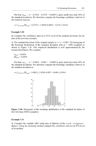
A: The standard deviation of the original sample is s ≡ w = 0.086. The histogram of
the bootstrap distribution of the standard deviation with m = 1000 resamples is
shown in Figure 3.10. This empirical distribution is well approximated by the
normal distribution. We compute:
w boot = 0.0854
SE boot = 0.0070
The bias w boot − w = 0.0854 – 0.086 = −0.0006 is quite small (less than 10% of
the standard deviation). We therefore compute the bootstrap confidence interval of
the standard deviation as:
w t ± 93 . 0 , 975 SE boot = 0.086 ± 1.9858×0.007 = 0.086 ± 0.014
300
n
250
200
150
100
50
w*
0
0.05 0.06 0.07 0.08 0.09 0.1 0.11
Figure 3.10. Histogram of the bootstrap distribution of the standard deviation of
the CaO data (1000 resamples).
Example 3.11
Q: Consider the variable ART (total area of defects) of the cork stoppers’
dataset. Using the bootstrap method compute the confidence interval at 95% level
of its median.