Page 132 - Applied Statistics Using SPSS, STATISTICA, MATLAB and R

112 4 Parametric Tests of Hypotheses

that the lifetime of the drills, X, for all the brands, follows a normal distribution
1
with the same standard deviation . We know, therefore, that the sampling
distribution of X is also normal with the following standard error (see sections 3.2
and A.8.4):

σ
σ = = 77 . 94 .
X
12
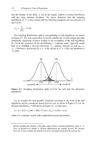
The sampling distributions (pdf’s) corresponding to both hypotheses are shown
in Figure 4.1. We seek a procedure to decide whether the 12-drill-sample provides
statistically significant evidence leading to the acceptance of the null hypothesis
H 0. Given the symmetry of the distributions, a “common sense” approach would
lead us to establish a decision threshold, x , halfway between µ A and µ B, i.e.
α
x =1200 hours, and decide H 0 if x >1200, decide H 1 if x <1200, and arbitrarily if
α
x =1200.

H 1 H 0

α β
x
1100 x α 1300
accept H 1 accept H 0
Figure 4.1. Sampling distribution (pdf) of X for the null and the alternative
hypotheses.

Let us consider the four possible situations according to the truth of the null
hypothesis and the conclusion drawn from the test, as shown in Figure 4.2. For the
decision threshold x =1200 shown in Figure 4.1, we then have:
α

α = β = P ( ≤ ( 1200 − 1300 / ) 77 . 94 ) = N 1 , 0 (− . 1 283 ) = . 0 10 ,
Z

where Z is a random varable with standardised normal distribution.

1
Strictly speaking the lifetime of the drills cannot follow a normal distribution, since X > 0.
Also, as discussed in chapter 9, lifetime distributions are usually skewed. We assume,
however, in this example, the distribution to be well approximated by the normal law.