Page 137 - Applied Statistics Using SPSS, STATISTICA, MATLAB and R

4.2 Test Errors and Test Power 117

x α = µ B − . 1 64×σ X = 1300 − . 1 64× 55 . 11 = 1209 6 . ,
which, compared with the previous value, is less deviated from µ B. The value of β
for µ A = 1100 is now:

β = P ( ≥ (x α − µ A / ) σ X ) = P ( ≥ ( 1209 6 . − 1100 / ) 55 . 11 ) = . 0 023 .
Z
Z

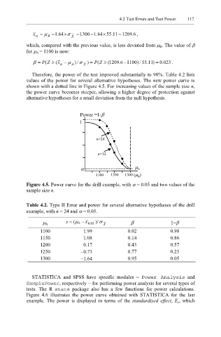
Therefore, the power of the test improved substantially to 98%. Table 4.2 lists
values of the power for several alternative hypotheses. The new power curve is
shown with a dotted line in Figure 4.5. For increasing values of the sample size n,
the power curve becomes steeper, allowing a higher degree of protection against
alternative hypotheses for a small deviation from the null hypothesis.

Power =1-β
1

n=24

n=12

α µ Α
1100 1200 1300 (µ )
B
Figure 4.5. Power curve for the drill example, with α = 0.05 and two values of the
sample size n.

Table 4.2. Type II Error and power for several alternative hypotheses of the drill
example, with n = 24 and α = 0.05.
µ A z = (µ A − x . 0 05 )/σ β 1−β
X
1100 1.99 0.02 0.98
1150 1.08 0.14 0.86
1200 0.17 0.43 0.57
1250 −0.73 0.77 0.23
1300 −1.64 0.95 0.05

STATISTICA and SPSS have specific modules − Power Analysis and
SamplePower , respectively − for performing power analysis for several types of
tests. The R stats package also has a few functions for power calculations.
Figure 4.6 illustrates the power curve obtained with STATISTICA for the last
example. The power is displayed in terms of the standardised effect, E s, which