Page 138 - Applied Statistics Using SPSS, STATISTICA, MATLAB and R

118 4 Parametric Tests of Hypotheses

measures the deviation of the alternative hypothesis from the null hypothesis,
normalised by the standard deviation, as follows:

µ − µ
E = B σ A . 4.1
s

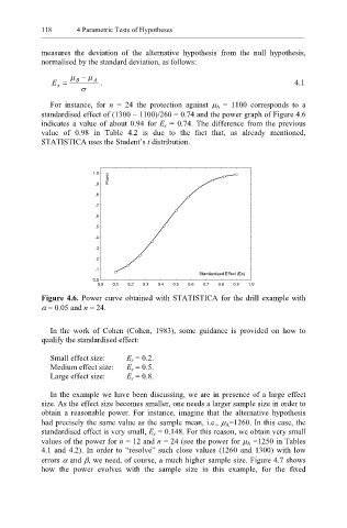
For instance, for n = 24 the protection against µ A = 1100 corresponds to a
standardised effect of (1300 − 1100)/260 = 0.74 and the power graph of Figure 4.6
indicates a value of about 0.94 for E s = 0.74. The difference from the previous
value of 0.98 in Table 4.2 is due to the fact that, as already mentioned,
STATISTICA uses the Student’s t distribution.

1.0
Power
.9
.8
.7
.6
.5
.4
.3
.2
.1
Standardized Effect (Es)
0.0
0.0 0.1 0.2 0.3 0.4 0.5 0.6 0.7 0.8 0.9 1.0
Figure 4.6. Power curve obtained with STATISTICA for the drill example with
α = 0.05 and n = 24.

In the work of Cohen (Cohen, 1983), some guidance is provided on how to
qualify the standardised effect:

Small effect size: E s = 0.2.
Medium effect size: E s = 0.5.
Large effect size: E s = 0.8.

In the example we have been discussing, we are in presence of a large effect
size. As the effect size becomes smaller, one needs a larger sample size in order to
obtain a reasonable power. For instance, imagine that the alternative hypothesis
had precisely the same value as the sample mean, i.e., µ A=1260. In this case, the
standardised effect is very small, E s = 0.148. For this reason, we obtain very small
values of the power for n = 12 and n = 24 (see the power for µ A =1250 in Tables
4.1 and 4.2). In order to “resolve” such close values (1260 and 1300) with low
errors α and β, we need, of course, a much higher sample size. Figure 4.7 shows
how the power evolves with the sample size in this example, for the fixed