Page 143 - Applied Statistics Using SPSS, STATISTICA, MATLAB and R

4.3 Inference on One Population 123

Example 4.1
Q: Consider the Meteo (meteorological) dataset (see Appendix E). Perform the
single mean test on the variable T81, representing the maximum temperature
registered during 1981 at several weather stations in Portugal. Assume that, based
on a large number of yearly records, a “typical” year has an average maximum
temperature of 37.5º, which will be used as the test value. Also, assume that the
Meteo dataset represents a random spatial sample and that the variable T81, for
the population of an arbitrarily large number of measurements performed in the
Portuguese territory, can be described by a normal distribution.
A: The purpose of the test is to assess whether or not 1981 was a “typical” year in
regard to average maximum temperature. We then formalise the single mean test
as:

H 0: µ T 81 = 37 5 . .
H 1: µ T 81 ≠ 37 5 . .

Table 4.3 lists the results that can be obtained either with SPSS or with
STATISTICA. The probability of obtaining a deviation from the test value, at least
as large as 39.8 – 37.5, is p ≈ 0. Therefore, the test is significant, i.e., the sample
does provide enough evidence to reject the null hypothesis at a very low α.
Notice that Table 4.3 also displays the values of t, the degrees of freedom,
df = n – 1, and the standard error s / n = 0.548.

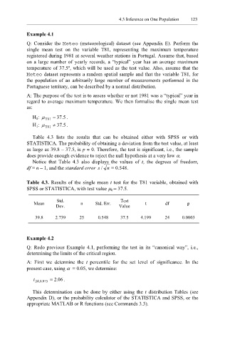
Table 4.3. Results of the single mean t test for the T81 variable, obtained with
SPSS or STATISTICA, with test value µ 0 = 37.5.

Std. Test
Mean n Std. Err. t df p
Dev. Value
39.8 2.739 25 0.548 37.5 4.199 24 0.0003

Example 4.2

Q: Redo previous Example 4.1, performing the test in its “canonical way”, i.e.,
determining the limits of the critical region.
A: First we determine the t percentile for the set level of significance. In the
present case, using α = 0.05, we determine:

t 24 . 0 , 975 = . 2 06 .

This determination can be done by either using the t distribution Tables (see
Appendix D), or the probability calculator of the STATISTICA and SPSS, or the
appropriate MATLAB or R functions (see Commands 3.3).