Page 145 - Applied Statistics Using SPSS, STATISTICA, MATLAB and R

4.3 Inference on One Population 125

When performing tests of hypotheses with MATLAB or R adequate percentiles
for the critical region, the so-called critical values, are also computed.
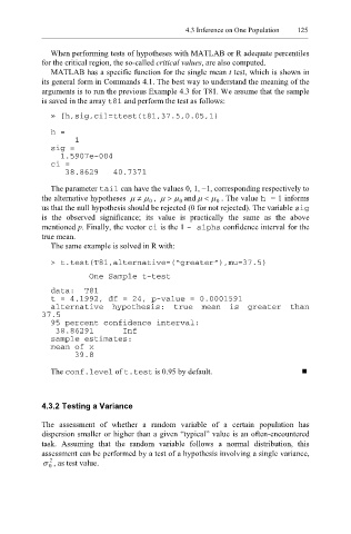
MATLAB has a specific function for the single mean t test, which is shown in
its general form in Commands 4.1. The best way to understand the meaning of the
arguments is to run the previous Example 4.3 for T81. We assume that the sample
is saved in the array t81 and perform the test as follows:

» [h,sig,ci]=ttest(t81,37.5,0.05,1)

h =
1
sig =
1.5907e-004
ci =
38.8629 40.7371

The parameter tail can have the values 0, 1, −1, corresponding respectively to
the alternative hypotheses µ ≠ µ , µ > µ and µ < µ . The value h = 1 informs
0
0
0
us that the null hypothesis should be rejected (0 for not rejected). The variable sig
is the observed significance; its value is practically the same as the above
mentioned p. Finally, the vector ci is the 1 - alpha confidence interval for the
true mean.
The same example is solved in R with:

> t.test(T81,alternative=(“greater”),mu=37.5)

One Sample t-test

data: T81
t = 4.1992, df = 24, p-value = 0.0001591
alternative hypothesis: true mean is greater than
37.5
95 percent confidence interval:
38.86291 Inf
sample estimates:
mean of x
39.8

The vel conf.le of t.tes t is 0.95 by default.

4.3.2 Testing a Variance

The assessment of whether a random variable of a certain population has
dispersion smaller or higher than a given “typical” value is an often-encountered
task. Assuming that the random variable follows a normal distribution, this
assessment can be performed by a test of a hypothesis involving a single variance,
2
σ , as test value.
0