Page 157 - Applied Statistics Using SPSS, STATISTICA, MATLAB and R

4.4 Inference on Two Populations 137

STATISTICA specification window needed for the power computation. Note the
specification of the one-sided hypothesis. Figure 4.10b shows that the power is
very high when the alternative hypothesis is formalised with population means
having the same values as the sample means; i.e., in this case the probability of
erroneously deciding H 0 is negligible. Note the computed value of the standardised
effect (µ 1 – µ 2)/s = 2.27, which is very large (see section 4.2).
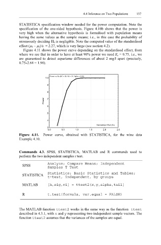
Figure 4.11 shows the power curve depending on the standardised effect, from
where we see that in order to have at least 90% power we need E s = 0.75, i.e., we
are guaranteed to detect aspartame differences of about 2 mg/l apart (precisely,
0.75×2.64 = 1.98).

Power vs. Es (N1 = 30, N2 = 37, Alpha = 0.05)
1.0
.9

.8
Power .7

.6
.5
.4
Standardized Effect (Es)
.3
0.0 0.5 1.0 1.5 2.0 2.5

Figure 4.11. Power curve, obtained with STATISTICA, for the wine data
Example 4.10.

Commands 4.3. SPSS, STATISTICA, MATLAB and R commands used to
perform the two independent samples t test.

SPSS Analyze; Compare Means; Independent
Samples T Test
STATISTICA Statistics; Basic Statistics and Tables;
t-test, independent, by groups
MATLAB [h,sig,ci] = ttest2(x,y,alpha,tail]

R t.test(formula, var.equal = FALSE)

The MATLAB function tte st2 works in the same way as the function ttest
described in 4.3.1, with x and y representing two independent sample vectors. The
function ttest2 assumes that the variances of the samples are equal.