Page 156 - Applied Statistics Using SPSS, STATISTICA, MATLAB and R

136 4 Parametric Tests of Hypotheses

For the variable ASP, we accept the null hypothesis of equal variances, since the
observed significance is very high (p = 0.896). We then look to the t test results in
the top row, which are based on the formulas 4.12 and 4.13. Note, particularly, that
the number of degrees of freedom is df = 30 + 37 – 2 = 65. According to the results
in the top row, we reject the null hypothesis of equal means with the observed
significance p = 0.022. As a matter of fact, we also reject the one-sided hypothesis
that aspartame content in white wines (sample mean 27.1 mg/l) is smaller or equal
to the content in red wines (sample mean 20.9 mg/l). Note that the means of the
two groups are more than two times the standard error apart.
For the variable PHE, we reject the hypothesis of equal variances; therefore, we
look to the t test results in the bottom row, which are based on formulas 4.14 and
4.15. The null hypothesis of equal means is also rejected, now with higher
significance since p = 0.002. Note that the means of the two groups are more than
three times the standard error apart.

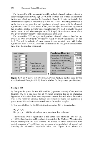
Figure 4.10. a) Window of STATISTICA Power Analysis module used for the
specifications of Example 4.10; b) Results window for the previous specifications.

Example 4.10
Q: Compute the power for the ASP variable (aspartame content) of the previous
Example 4.9, for a one-sided test at 5% level, assuming that as an alternative
hypothesis white wines have more aspartame content than red wines. Determine
what is the minimum distance between the population means that guarantees a
power above 90% under the same conditions as the studied samples.
A: The one-sided test for this RS situation (see section 4.2) is formalised as:

H 0: µ 1 ≤ µ 2;
H 1: µ 1 > µ 2 . (White wines have more aspartame than red wines.)

The observed level of significance is half of the value shown in Table 4.6, i.e.,
p = 0.011; therefore, the null hypothesis is rejected at the 5% level. When the data
analyst investigated the ASP variable, he wanted to draw conclusions with
protection against a Type II Error, i.e., he wanted a low probability of wrongly not
detecting the alternative hypothesis when true. Figure 4.10a shows the