Page 159 - Applied Statistics Using SPSS, STATISTICA, MATLAB and R

4.4 Inference on Two Populations 139

> power.t.test(30, delta=NULL, 2.64, power=0.9,
type=c(“two.sample”),alternative=c(“one.sided”))

The result delta = 2 would be obtained exactly as we found out in Figure
4.11.

4.4.3.3 Testing Means on Paired Samples

As explained in 4.4.3.1, given the sets x = [x 1 x 2 … x n]’ and y = [y 1 y 2 … y n]’, where
the x i, y i refer to objects that can be paired, we then compute the paired differences:
d 1 = y 1 – x 1, d 2 = y 2 – x 2, …, d n = y n – x n. Therefore, the null hypothesis:

H 0: µ X = µ Y,

is rewritten as:

H 0: µ D = 0 with D = X – Y .

The test is, therefore, converted into a single mean t test, using the studentised
statistic:

t * = d ~ t n 1 − , 4.16
s d / n

where s d is the sample estimate of the variance of D, computed with the differences
d i. Note that since X and Y are not independent the additive property of the
variances does not apply (see formula A.58c).

Example 4.11
Q: Consider the meteorological dataset. Use an appropriate test in order to compare
the maximum temperatures of the year 1980 with those of the years 1981 and
1982.
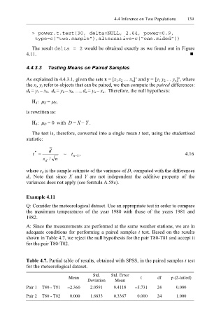
A: Since the measurements are performed at the same weather stations, we are in
adequate conditions for performing a paired samples t test. Based on the results
shown in Table 4.7, we reject the null hypothesis for the pair T80-T81 and accept it
for the pair T80-T82.

Table 4.7. Partial table of results, obtained with SPSS, in the paired samples t test
for the meteorological dataset.

Std. Std. Error
Mean t df p (2-tailed)
Deviation Mean
Pair 1 T80 - T81 −2.360 2.0591 0.4118 −5.731 24 0.000
Pair 2 T80 - T82 0.000 1.6833 0.3367 0.000 24 1.000