Page 155 - Applied Statistics Using SPSS, STATISTICA, MATLAB and R

4.4 Inference on Two Populations 135

Then, the following test statistic:

x − x
*
t = A B , 4.14
s A 2 + s 2 B
n A n B

has a Student’s t distribution with the following degrees of freedom:

(s 2 / n + s 2 / n ) 2
df = A A B B . 4.15
(s A 2 / n A ) 2 / n + (s B 2 / n B ) 2 / n B
A

In order to decide which case to consider – equal or unequal variances – the F
test or Levene’s test, described in section 4.4.2, are performed. SPSS and
STATISTICA do precisely this.

Example 4.9
Q: Consider the Wines’ dataset (see description in Appendix E). Test at a 5%
level of significance whether the variables ASP (aspartame content) and PHE
(phenylalanine content) can distinguish white wines from red wines. The collected
samples are assumed to be random. The distributions of ASP and PHE are well
approximated by the normal distribution in both populations (white and red wines).
The samples are described by the grouping variable TYPE (1 = white; 2 = red) and
their sizes are n 1 = 30 and n 2 = 37, respectively.
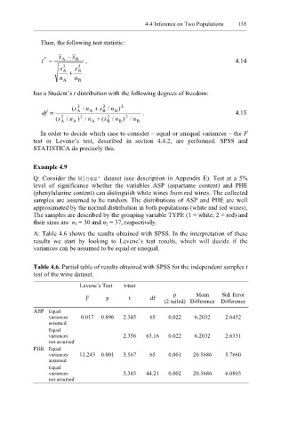
A: Table 4.6 shows the results obtained with SPSS. In the interpretation of these
results we start by looking to Levene’s test results, which will decide if the
variances can be assumed to be equal or unequal.

Table 4.6. Partial table of results obtained with SPSS for the independent samples t
test of the wine dataset.
Levene’s Test t-test
p Mean Std. Error
F p t df
(2-tailed) Difference Difference
ASP Equal
variances 0.017 0.896 2.345 65 0.022 6.2032 2.6452
assumed
Equal
variances 2.356 63.16 0.022 6.2032 2.6331
not assumed
PHE Equal
variances 11.243 0.001 3.567 65 0.001 20.5686 5.7660
assumed
Equal
variances 3.383 44.21 0.002 20.5686 6.0803
not assumed