Page 242 - Applied Statistics Using SPSS, STATISTICA, MATLAB and R

6 Statistical Classification

Statistical classification deals with rules of case assignment to categories or
classes. The classification, or decision rule, is expressed in terms of a set of
random variables − the case features. In order to derive the decision rule, one
assumes that a training set of pre-classified cases − the data sample − is available,
and can be used to determine the sought after rule applicable to new cases. The
decision rule can be derived in a model-based approach, whenever a joint
distribution of the random variables can be assumed, or in a model-free approach,
otherwise.

6.1 Decision Regions and Functions

Consider a data sample constituted by n cases, depending on d features. The central
idea in statistical classification is to use the data sample, represented by vectors in
d
an ℜ feature space, in order to derive a decision rule that partitions the feature
space into regions assigned to the classification classes. These regions are called
decision regions. If a feature vector falls into a certain decision region, the
associated case is assigned to the corresponding class.
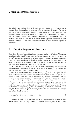
Let us assume two classes, ω 1 and ω 2, of cases described by two-dimensional
feature vectors (coordinates x 1 and x 2) as shown in Figure 6.1. The features are
random variables, X 1 and X 2, respectively.
] ∈
2
Each case is represented by a vector x = [x 1 x ’ ℜ . In Figure 6.1, we
2
used o to denote class ω 1 cases and × to denote class ω 2 cases. In general, the
“ ”
“ ”
cases of each class will be characterised by random distributions of the
corresponding feature vectors, as illustrated in Figure 6.1, where the ellipses
represent equal-probability density curves that enclose most of the cases.
Figure 6.1 also shows a straight line separating the two classes. We can easily
write the equation of the straight line in terms of the features X 1, X 2 using
coefficients or weights w 1, w 2 and a bias term w 0 as shown in equation 6.1. The
weights determine the slope of the straight line; the bias determines the straight
line intersect with the axes.

d X , 1 X 2 (x ) ≡ ( d x ) = w 1 x 1 + w 2 x 2 + w 0 = 0 . 6.1

Equation 6.1 also allows interpretation of the straight line as the root set of a
linear function d(x). We say that d(x) is a linear decision function that divides