Page 245 - Applied Statistics Using SPSS, STATISTICA, MATLAB and R

226 6 Statistical Classification

Equation 6.6c, linear in x, represents a hyperplane perpendicular to (m 1 – m 2)’
and passing through the point 0.5(m 1 + m 2)’ halfway between the means, as
illustrated in Figure 6.1 for d = 2 (the hyperplane is then a straight line).
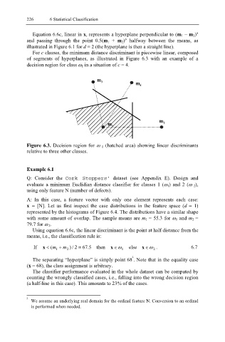
For c classes, the minimum distance discriminant is piecewise linear, composed
of segments of hyperplanes, as illustrated in Figure 6.3 with an example of a
decision region for class ω 1 in a situation of c = 4.

m 3
m
4

m
m 1 2

Figure 6.3. Decision region for ω 1 (hatched area) showing linear discriminants
relative to three other classes.

Example 6.1

Q: Consider the Cork Stoppers’ dataset (see Appendix E). Design and
evaluate a minimum Euclidian distance classifier for classes 1 (ω 1) and 2 (ω 2),
using only feature N (number of defects).
A: In this case, a feature vector with only one element represents each case:
x = [N]. Let us first inspect the case distributions in the feature space (d = 1)
represented by the histograms of Figure 6.4. The distributions have a similar shape
with some amount of overlap. The sample means are m 1 = 55.3 for ω 1 and m 2 =
79.7 for ω 2.
Using equation 6.6c, the linear discriminant is the point at half distance from the
means, i.e., the classification rule is:

If x < (m 1 + m 2 2 / ) = 67 5 . then x ∈ ω 1 else x ∈ ω . 6.7
2

2
The separating “hyperplane” is simply point 68 . Note that in the equality case
(x = 68), the class assignment is arbitrary.
The classifier performance evaluated in the whole dataset can be computed by
counting the wrongly classified cases, i.e., falling into the wrong decision region
(a half-line in this case). This amounts to 23% of the cases.

2
We assume an underlying real domain for the ordinal feature N. Conversion to an ordinal
is performed when needed.