Page 249 - Applied Statistics Using SPSS, STATISTICA, MATLAB and R

230 6 Statistical Classification

linking the means. The only difference from the results of the previous section is
that the hyperplanes separating class ω i from class ω j are now orthogonal to the
-1
vector Σ (m i − m j).
In practice, it is impossible to guarantee that all class covariance matrices are
equal. Fortunately, the decision surfaces are usually not very sensitive to mild
deviations from this condition; therefore, in normal practice, one uses an estimate
of a pooled covariance matrix, computed as an average of the sample covariance
matrices. This is the practice followed by SPSS and STATISTICA.

Example 6.3
Q: Redo Example 6.1, using a minimum Mahalanobis distance classifier. Check
the computation of the discriminant parameters and determine to which class a
cork with 65 defects is assigned.

A: Given the similarity of both distributions, the Mahalanobis classifier produces
the same classification results as the Euclidian classifier. Table 6.1 shows the
classification matrix (obtained with SPSS) with the predicted classifications along
the columns and the true (observed) classifications along the rows. We see that for
this simple classifier, the overall percentage of correct classification in the data
sample (training set) is 77%, or equivalently, the overall training set error is 23%
(18% for ω 1 and 28% for ω 2). For the moment, we will not assess how the
classifier performs with independent cases, i.e., we will not assess its test set error.
The decision function coefficients (also known as Fisher’s coefficients), as
computed by SPSS, are shown in Table 6.2.

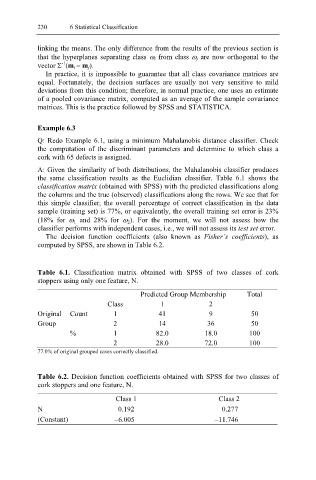
Table 6.1. Classification matrix obtained with SPSS of two classes of cork
stoppers using only one feature, N.
Predicted Group Membership Total
Class 1 2
Original Count 1 41 9 50
Group 2 14 36 50
% 1 82.0 18.0 100
2 28.0 72.0 100
77.0% of original grouped cases correctly classified.

Table 6.2. Decision function coefficients obtained with SPSS for two classes of
cork stoppers and one feature, N.
Class 1 Class 2
N 0.192 0.277
(Constant) −6.005 −11.746