Page 254 - Applied Statistics Using SPSS, STATISTICA, MATLAB and R

6.3 Bayesian Classification 235

Note that the prevalences are not entirely controlled by the factory, and that they
depend mainly on the quality of the raw material. Just as, likewise, a cardiologist
cannot control how prevalent myocardial infarction is in a given population.
Prevalences can, therefore, be regarded as “states of nature”.
Suppose we are asked to make a blind decision as to which class a cork stopper
belongs without looking at it. If the only available information is the prevalences,
the sensible choice is class ω 2. This way, we expect to be wrong only 40% of the
times.
Assume now that we were allowed to measure the feature vector x of the
presented cork stopper. Let (P ω i | ) x be the conditional probability of the cork
stopper represented by x belonging to class ω i. If we are able to determine the
P
probabilities (ωP 1 | ) x and (ω 2 | ) x , the sensible decision is now:

P
If (ωP 1 | ) x > (ω 2 | ) x we decide x ∈ ω ;
1
P
If (ωP 1 | ) x < (ω 2 | ) x we decide x ∈ ω ; 6.15
2
P
If (ωP 1 | ) x = (ω 2 | ) x the decision is arbitrary.

We can condense 6.15 as:

If (ωP 1 | ) x > (ω 2 | ) x then ∈ ω else ∈ ω . 6.15a
x
P
x
2
1

The posterior probabilities (P ω i | ) x can be computed if we know the pdfs of
the distributions of the feature vectors in both classes, p (x |ω i ) , the so-called
likelihood of x. As a matter of fact, the Bayes law (see Appendix A) states that:

p (x |ω )P (ω )
( P ω i | ) x = i i , 6.16
p (x )
with p )(x = ∑ c = i 1 p( ω i ) P(ω i ) , the total probability of x.
|
x
Note that P(ω i) and P(ω i | x) are discrete probabilities (symbolised by a capital
letter), whereas p(x |ω i) and p(x) are values of pdf functions. Note also that the
term p(x) is a common term in the comparison expressed by 6.15a, therefore, we
may rewrite for two classes:

x
|
x
x
If ( ωp x | 1 )P (ω 1 ) > ( ω 2 )P (ω 2 ) then ∈ ω else ∈ ω , 6.17
p
1
2

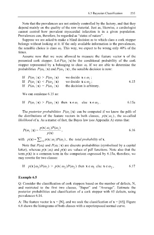
Example 6.5
Q: Consider the classification of cork stoppers based on the number of defects, N,
and restricted to the first two classes, “Super” and “Average”. Estimate the
posterior probabilities and classification of a cork stopper with 65 defects, using
prevalences 6.14.
A: The feature vector is x = [N], and we seek the classification of x = [65]. Figure
6.8 shows the histograms of both classes with a superimposed normal curve.