Page 250 - Applied Statistics Using SPSS, STATISTICA, MATLAB and R

6.2 Linear Discriminants 231

Let us check these results. The class means are m 1 = [55.28] and m 2 = [79.74].
2
The average variance is s = 287.63. Applying formula 6.10d we obtain:

w 1 = m 1 2 = [ / s . 0 ] 192 ; w 0 , 1 = − 5 . 0 m 1 2 / s 2 = − . 6 005. 6.11a
w 2 = m 2 2 = [ / s . 0 ] 277 ; w 0 , 2 = − 5 . 0 m 2 2 / s 2 = − 11 . 746 . 6.11b

These results confirm the ones shown in Table 6.2. Let us determine the class
assignment of a cork-stopper with 65 defects. As g 1([65]) = 0.192×65 – 6.005 =
6.48 is greater than g 2([65]) = 0.227×65 – 11.746 = 6.26 it is assigned to class ω 1.

Example 6.4
Q: Redo Example 6.2, using a minimum Mahalanobis distance classifier. Check
the computation of the discriminant parameters and determine to which class a
cork with 65 defects and with a total perimeter of 520 pixels (PRT10 = 52) is
assigned.
A: The training set classification matrix is shown in Table 6.3. A significant
improvement was obtained in comparison with the Euclidian classifier results
mentioned in section 6.2.1; namely, an overall training set error of 10% instead of
18%. The Mahalanobis distance, taking into account the shape of the data clusters,
not surprisingly, performed better. The decision function coefficients are shown in
Table 6.4. Using these coefficients, we write the decision functions as:

] 262 −
g 1 (x 1 x + w 0 , 1 = [) = w ’ . 0 . 0 09783 x − . 6 138 . 6.12a
] 0803
g 2 (x 2 x + w 0 , 2 = [ ) = w ’ . 0 . 0 2776 x − 12 . 817 . 6.12b

The point estimate of the pooled covariance matrix of the data is:

 287 . 63 204 . 070   .0 0216 − 0255.0 
S =   ⇒ S −1 =   . 6.13
 204 . 070 172 . 553   − 0255.0 . 0 036 

-1
Substituting S in formula 6.10d, the results shown in Table 6.4 are obtained.

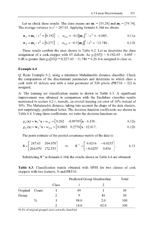
Table 6.3. Classification matrix obtained with SPSS for two classes of cork
stoppers with two features, N and PRT10.

Predicted Group Membership Total
Class 1 2
Original Count 1 49 1 50
Group 2 9 41 50
% 1 98.0 2.0 100
2 18.0 82.0 100
90.0% of original grouped cases correctly classified.