Page 251 - Applied Statistics Using SPSS, STATISTICA, MATLAB and R

232 6 Statistical Classification

-1
’
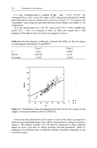
It is also straightforward to compute S (m 1 − m 2) = [0.18 −0.376] . The
orthogonal line to this vector with slope 0.4787 and passing through the middle
point between the means is shown with a solid line in Figure 6.7. As expected, the
“hyperplane” leans along the regression direction of the features (see Figure 6.5 for
comparison).
As to the classification of x = [65 52]’, since g ([65 52]’) = 5.80 is smaller than
1
g 2([65 52] ) = 6.86, it is assigned to class ω 2. This cork stopper has a total
’
perimeter of the defects that is too big to be assigned to class ω 1.

Table 6.4. Decision function coefficients, obtained with SPSS, for the two classes
of cork stoppers with features N and PRT10.
Class 1 Class 2
N 0.262 0.0803
PRT10 -0.09783 0.278
(Constant) -6.138 -12.817

Figure 6.7. Mahalanobis linear discriminant (solid line) for the two classes of cork
stoppers. Scatter plot obtained with STATISTICA.

Notice that if the distributions of the feature vectors in the classes correspond to
different hyperellipsoidal shapes, they will be characterised by unequal covariance
matrices. The distance formula 6.10 will then be influenced by these different
shapes in such a way that we obtain quadratic decision boundaries. Table 6.5
summarises the different types of minimum distance classifiers, depending on the
covariance matrix.