Page 248 - Applied Statistics Using SPSS, STATISTICA, MATLAB and R

6.2 Linear Discriminants 229

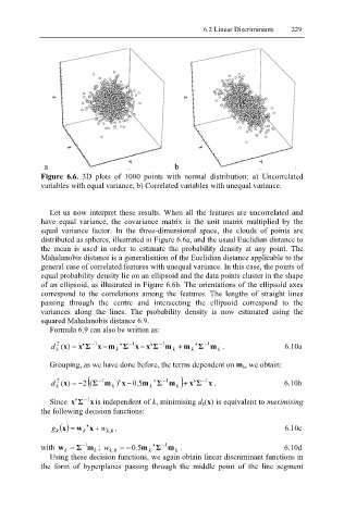
Figure 6.6. 3D plots of 1000 points with normal distribution: a) Uncorrelated
variables with equal variance; b) Correlated variables with unequal variance.

Let us now interpret these results. When all the features are uncorrelated and
have equal variance, the covariance matrix is the unit matrix multiplied by the
equal variance factor. In the three-dimensional space, the clouds of points are
distributed as spheres, illustrated in Figure 6.6a, and the usual Euclidian distance to
the mean is used in order to estimate the probability density at any point. The
Mahalanobis distance is a generalisation of the Euclidian distance applicable to the
general case of correlated features with unequal variance. In this case, the points of
equal probability density lie on an ellipsoid and the data points cluster in the shape
of an ellipsoid, as illustrated in Figure 6.6b. The orientations of the ellipsoid axes
correspond to the correlations among the features. The lengths of straight lines
passing through the centre and intersecting the ellipsoid correspond to the
variances along the lines. The probability density is now estimated using the
squared Mahalanobis distance 6.9.
Formula 6.9 can also be written as:

2
d ( x) = x’ Σ − 1 x − m ’ Σ − 1 x − x’ Σ − 1 m + m ’ Σ − 1 m . 6.10a
k
k
k
k
k

Grouping, as we have done before, the terms dependent on m k, we obtain:

−
d 2 k ( x) = − 2 ( Σ( − 1 m )’ x 0 5 . m ’ Σ − 1 m k ) x+ ’ Σ − 1 x . 6.10b
k
k

Since x’ Σ − 1 x is independent of k, minimising d k(x) is equivalent to maximising
the following decision functions:

g k () = wx k x ’ + w 0 , k , 6.10c

with w = Σ − 1 m ; w k 0, = − 5 . 0 m ’ Σ − 1 m . 6.10d
k
k
k
k
Using these decision functions, we again obtain linear discriminant functions in
the form of hyperplanes passing through the middle point of the line segment