Page 243 - Applied Statistics Using SPSS, STATISTICA, MATLAB and R

224 6 Statistical Classification

2
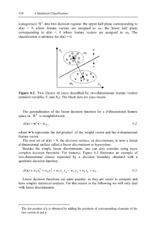
(categorises) ℜ into two decision regions: the upper half plane corresponding to
d(x) > 0 where feature vectors are assigned to ω 1; the lower half plane
corresponding to d(x) < 0 where feature vectors are assigned to ω 2. The
classification is arbitrary for d(x) = 0.

x 2 ω +
o o o o o 1
o o o o
o
o o
-
x x x x
x x x x x
x
ω 2 x
1

Figure 6.1. Two classes of cases described by two-dimensional feature vectors
(random variables X 1 and X 2). The black dots are class means.

The generalisation of the linear decision function for a d-dimensional feature
d
space in ℜ is straightforward:

d (x ) = w’ x + w , 6.2
0

1
where w x represents the dot product of the weight vector and the d-dimensional
’
feature vector.
The root set of d(x) = 0, the decision surface, or discriminant, is now a linear
d-dimensional surface called a linear discriminant or hyperplane.
Besides the simple linear discriminants, one can also consider using more
complex decision functions. For instance, Figure 6.2 illustrates an example of
two-dimensional classes separated by a decision boundary obtained with a
quadratic decision function:

2
2
( d x ) = w 5 x + w 4 x + w 3 x 1 x + w 2 x + w 1 x + w 0 . 6.3
1
2
1
2
2

Linear decision functions are quite popular, as they are easier to compute and
have simpler statistical analysis. For this reason in the following we will only deal
with linear discriminants.

1
’
The dot product x y is obtained by adding the products of corresponding elements of the
two vectors x and y.