Page 244 - Applied Statistics Using SPSS, STATISTICA, MATLAB and R

6.2 Linear Discriminants 225

x 2 o o
o o o o o o o ω
o
o o o o 2
o oo o o o
o o o o o
x
o o x x x x x x x
x x
x x
x
x x
x
o x x x x x x x x x ω 1
x
x
x
x x x x x x x
x x x x 1

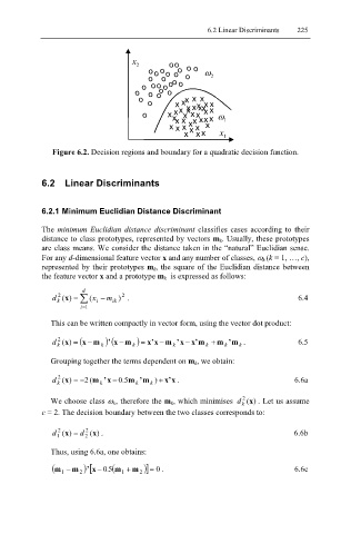
Figure 6.2. Decision regions and boundary for a quadratic decision function.
6.2 Linear Discriminants
6.2.1 Minimum Euclidian Distance Discriminant

The minimum Euclidian distance discriminant classifies cases according to their
distance to class prototypes, represented by vectors m k. Usually, these prototypes
are class means. We consider the distance taken in the “natural” Euclidian sense.
For any d-dimensional feature vector x and any number of classes, ω k (k = 1, …, c),
represented by their prototypes m k, the square of the Euclidian distance between
the feature vector x and a prototype m k is expressed as follows:

d
2
2
d (x ) = ∑ x ( i − m ) . 6.4
k
ik
= i 1

This can be written compactly in vector form, using the vector dot product:

2
=
d ( x = (x − m k )(x − m k ) x’ x − m ’ x − x’ m + m ’ m . 6.5
’
)
k
k
k
k
k

Grouping together the terms dependent on m k, we obtain:

d 2 k ( x = − ( m ’ x − 5 m ’ m ) + x’ x . 6.6a
0
2
)
.
k
k
k

We choose class ω k, therefore the m k, which minimises d k 2 (x ) . Let us assume
c = 2. The decision boundary between the two classes corresponds to:

d 1 2 (x ) = d 2 2 (x ) . 6.6b

Thus, using 6.6a, one obtains:

( 1 −m 2 )m ’ x 0. ( [ 1 + m 2 ) 5 m ] − = 0 . 6.6c