Page 255 - Applied Statistics Using SPSS, STATISTICA, MATLAB and R

236 6 Statistical Classification

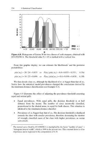
Figure 6.8. Histograms of feature N for two classes of cork stoppers, obtained with
STATISTICA. The threshold value N = 65 is marked with a vertical line.

3
From this graphic display, we can estimate the likelihoods and the posterior
probabilities:

p (x |ω 1 ) = 20 / 24 = . 0 833 ⇒ P (ω 1 ) p (x |ω 1 ) = 4 . 0 × . 0 833 = . 0 333 ; 6.18a
p (x |ω 2 ) = 16 / 23 = . 0 696 ⇒ P (ω 2 ) p (x |ω 2 ) = 6 . 0 × . 0 696 = . 0 418. 6.18b

We then decide class ω 2, although the likelihood of ω 1 is bigger than that of ω 2 .
Notice how the statistical model prevalences changed the conclusions derived by
the minimum distance classification (see Example 6.3).

Figure 6.9 illustrates the effect of adjusting the prevalence threshold assuming
equal and normal pdfs:

• Equal prevalences. With equal pdfs, the decision threshold is at half
distance from the means. The number of cases incorrectly classified,
proportional to the shaded areas, is equal for both classes. This situation is
identical to the minimum distance classifier.
• Prevalence of ω 1 bigger than that of ω 2. The decision threshold is displaced
towards the class with smaller prevalence, therefore decreasing the number
of wrongly classified cases of the class with higher prevalence, as seems
convenient.

3
The normal curve fitted by STATISTICA is multiplied by the factor “number of cases” ×
“ histogram interval width”, which is 1000 in the present case. This constant factor is of no
importance and is neglected in the computations of 6.18.