Page 257 - Applied Statistics Using SPSS, STATISTICA, MATLAB and R

238 6 Statistical Classification

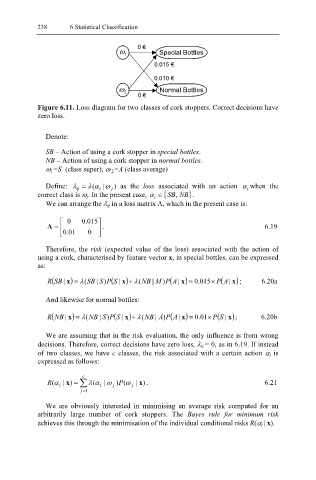
ω 1 0 € Special Bottles

0.015 €
0.010 €
ω 2 Normal Bottles
0 €
Figure 6.11. Loss diagram for two classes of cork stoppers. Correct decisions have
zero loss.

Denote:

SB – Action of using a cork stopper in special bottles.
NB – Action of using a cork stopper in normal bottles.
ω 1=S (class super); ω 2=A (class average)

Define: λ = λ (α i |ω j ) as the loss associated with an action α when the
ij
i
correct class is ω j. In the present case, α i ∈ {SB, NB }.
We can arrange the λ ij in a loss matrix Λ, which in the present case is:

 0 . 0 015 
Λ =   . 6.19
 . 0 01 0 

Therefore, the risk (expected value of the loss) associated with the action of
using a cork, characterised by feature vector x, in special bottles, can be expressed
as:

×
R ( x | )SB = λ (SB ( | S x | S ) )P + λ (NB | M )P ( |A ) x = . 0 015 P ( |A ) x ; 6.20a

And likewise for normal bottles:

×
R ( x | )NB = λ (NB ( | S x | S ) )P + λ (NB | A )P ( |A ) x = . 0 01 P ( |S ) x ; 6.20b

We are assuming that in the risk evaluation, the only influence is from wrong
decisions. Therefore, correct decisions have zero loss, λ ii = 0, as in 6.19. If instead
of two classes, we have c classes, the risk associated with a certain action α i is
expressed as follows:

c
R(α i | ) x = ∑ (αλ i |ω j ) P(ω j | ) x . 6.21
= j 1

We are obviously interested in minimising an average risk computed for an
arbitrarily large number of cork stoppers. The Bayes rule for minimum risk
achieves this through the minimisation of the individual conditional risks R(α i | x).