Page 260 - Applied Statistics Using SPSS, STATISTICA, MATLAB and R

6.3 Bayesian Classification 241

Note that even when the data distributions are not normal, as long as they are
symmetric and in correspondence to ellipsoidal shaped clusters of points, we obtain
the same decision surfaces as for a normal classifier, although with different error
rates and posterior probabilities.
As previously mentioned SPSS and STATISTICA use a pooled covariance
matrix when performing linear discriminant analysis. The influence of this practice
on the obtained error, compared with the theoretical optimal Bayesian error
corresponding to a quadratic classifier, is discussed in detail in (Fukunaga, 1990).
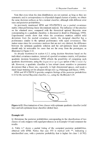
Experimental results show that when the covariance matrices exhibit mild
deviations from the pooled covariance matrix, the designed classifier has a
performance similar to the optimal performance with equal covariances. This
makes sense since for covariance matrices that are not very distinct, the difference
between the optimum quadratic solution and the sub-optimum linear solution
should only be noticeable for cases that are far away from the prototypes, as
illustrated in Figure 6.12.
As already mentioned in section 6.2.3, using decision functions based on the
individual covariance matrices, instead of a pooled covariance matrix, will produce
quadratic decision boundaries. SPSS affords the possibility of computing such
quadratic discriminants, using the Separate-groups option of the C lassify
tab. However, a quadratic classifier is less robust (more sensitive to parameter
deviations) than a linear one, especially in high dimensional spaces, and needs a
much larger training set for adequate design (see e.g. Fukunaga and Hayes, 1989).
SPSS and STATISTICA provide complete listings of the posterior probabilities
6.18 for the normal Bayesian classifier, i.e., using the likelihoods 6.24.

x 2

x 1

Figure 6.12. Discrimination of two classes with optimum quadratic classifier (solid
line) and sub-optimum linear classifier (dotted line).

Example 6.8
Q: Determine the posterior probabilities corresponding to the classification of two
classes of cork stoppers with equal prevalences as in Example 6.4 and comment the
results.
A: Table 6.7 shows a partial listing of the computed posterior probabilities,
obtained with SPSS. Notice that case #55 is marked with **, indicating a
misclassified case, with a posterior probability that is higher for class 1 (0.782)