Page 263 - Applied Statistics Using SPSS, STATISTICA, MATLAB and R

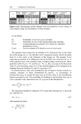
244 6 Statistical Classification

Figure 6.14. Classification results obtained with STATISTICA, of two classes of
cork stoppers using: (a) Ten features; (b) Four features.

Let us denote:

Pe – Probability of error of a given classifier;
Pe * – Probability of error of the optimum Bayesian classifier;
Pe d (n) – Training (design) set estimate of Pe based on a classifier
designed on n cases;
Pe t (n) – Test set estimate of Pe based on a set of n test cases.

The quantity Pe d (n) represents an estimate of Pe influenced only by the finite
size of the design set, i.e., the classifier error is measured exactly, and its deviation
from Pe is due solely to the finiteness of the design set. The quantity Pe t(n)
represents an estimate of Pe influenced only by the finite size of the test set, i.e., it
is the expected error of the classifier when evaluated using n-sized test sets. These
quantities verify Pe d (∞) = Pe and Pe t (∞) = Pe, i.e., they converge to the theoretical
value Pe with increasing values of n. If the classifier happens to be designed as an
*
optimum Bayesian classifier Pe d and Pe t converge to Pe .
In normal practice, these error probabilities are not known exactly. Instead, we
compute estimates of these probabilities, eP ˆ d and P ˆ e , as percentages of
t
misclassified cases, in exactly the same way as we have done in the classification
matrices presented so far. The probability of obtaining k misclassified cases out of
n for a classifier with a theoretical error Pe, is given by the binomial law:

 n
k
P( k =)     Pe 1( − Pe) n− k . 6.26
 k 

The maximum likelihood estimation of Pe under this binomial law is precisely
(see Appendix C):

P ˆ e = k n / , 6.27

with standard deviation:

Pe 1− Pe)
(
σ = . 6.28
n