Page 267 - Applied Statistics Using SPSS, STATISTICA, MATLAB and R

248 6 Statistical Classification

We then proceed to determine for every possible threshold value, ∆, the
sensitivity and specificity of the decision rule in the classification of the students.
These computations are summarised in Table 6.9.
Note that when Δ = 0 the decision rule assigns all students to the “Pass” group
(all students have AB ≥ 0). For 0 < Δ ≤ 1 the decision rule assigns to the “Pass”
group 135 students that have indeed “passed” and 60 students that have “flunked”
(these 195 students have AB ≥ 1). Likewise for other values of ∆ up to ∆ > 2 where
the decision rule assigns all students to the flunk group since no students have
∆ > 2. Based on the classification matrices for each value of ∆ the sensitivities and
specificities are computed as shown in Table 6.9.
The ROC curve can be directly drawn using these computations, or using SPSS
as shown in Figure 6.17c. Figures 6.17a and 6.17b show how the data must be
specified. From visual inspection, we see that the ROC curve is only moderately
off the diagonal, corresponding to a non-informative decision rule (more details,
later).

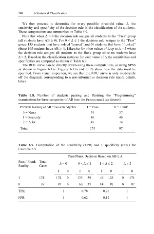
Table 6.8. Number of students passing and flunking the “Programming”
examination for three categories of AB (see the Programming dataset).
Previous learning of AB = Boolean Algebra 1 = Pass 0 = Flunk
0 = None 39 37
1 = Scarcely 86 46
2 = A lot 49 14
Total 174 97

Table 6.9. Computation of the sensitivity (TPR) and 1−specificity (FPR) for
Example 6.9.

Pass/Flunk Decision Based on AB ≥ ∆
Pass / Flunk Total ∆ = 0 0 < ∆ ≤ 1 1 < ∆ ≤ 2 ∆ > 2
Reality Cases
1 0 1 0 1 0 1 0
1 174 174 0 135 39 49 125 0 174

0 97 97 0 60 37 14 83 0 97
TPR 1 0.78 0.28 0

FPR 1 0.62 0.14 0