Page 270 - Applied Statistics Using SPSS, STATISTICA, MATLAB and R

6.4 The ROC Curve 251

In order to obtain the best threshold, we minimise the risk R by differentiating
and equalling to zero, obtaining then:

ds (∆ ) = (λ nn − λ na )P (N ) . 6.29
df (∆ ) (λ aa − λ an )P ( ) A

The point of the ROC curve where the slope has the value given by formula
6.29 represents the optimum operating point or, in other words, corresponds to the
best threshold for the two-class problem. Notice that this is a model-free technique
of choosing a feature threshold for discriminating two classes, with no assumptions
concerning the specific distributions of the cases.

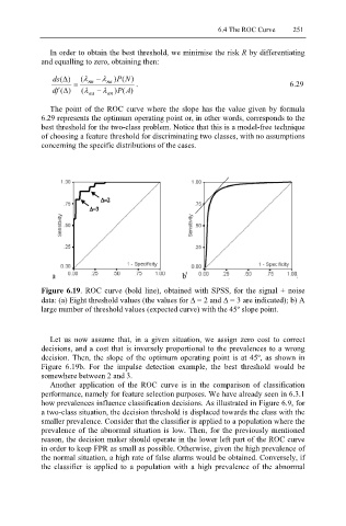
Figure 6.19. ROC curve (bold line), obtained with SPSS, for the signal + noise
data: (a) Eight threshold values (the values for ∆ = 2 and ∆ = 3 are indicated); b) A
large number of threshold values (expected curve) with the 45º slope point.

Let us now assume that, in a given situation, we assign zero cost to correct
decisions, and a cost that is inversely proportional to the prevalences to a wrong
decision. Then, the slope of the optimum operating point is at 45º, as shown in
Figure 6.19b. For the impulse detection example, the best threshold would be
somewhere between 2 and 3.
Another application of the ROC curve is in the comparison of classification
performance, namely for feature selection purposes. We have already seen in 6.3.1
how prevalences influence classification decisions. As illustrated in Figure 6.9, for
a two-class situation, the decision threshold is displaced towards the class with the
smaller prevalence. Consider that the classifier is applied to a population where the
prevalence of the abnormal situation is low. Then, for the previously mentioned
reason, the decision maker should operate in the lower left part of the ROC curve
in order to keep FPR as small as possible. Otherwise, given the high prevalence of
the normal situation, a high rate of false alarms would be obtained. Conversely, if
the classifier is applied to a population with a high prevalence of the abnormal