Page 271 - Applied Statistics Using SPSS, STATISTICA, MATLAB and R

252 6 Statistical Classification

situation, the decision-maker should adjust the decision threshold to operate on the
FPR high part of the curve.
Briefly, in order for our classification method to perform optimally for a large
range of prevalence situations, we would like to have an ROC curve very near the
perfect curve, i.e., with an underlying area of 1. It seems, therefore, reasonable to
select from among the candidate classification methods (or features) the one that
has an ROC curve with the highest underlying area.
The area under the ROC curve is computed by the SPSS with a 95% confidence
interval.
Despite some shortcomings, the ROC curve area method is a popular method of
assessing classifier or feature performance. This and an alternative method based
on information theory are described in Metz et al. (1973).

Commands 6.2. SPSS command used to perform ROC curve analysis.

SPSS Graphs; ROC Curve

Example 6.11

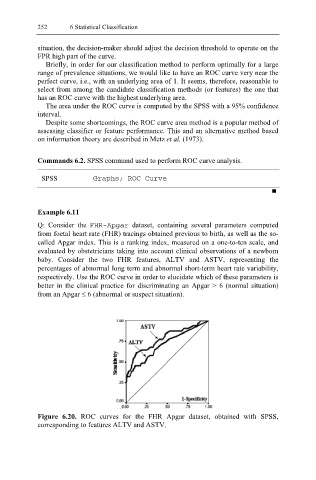
Q: Consider the FHR-Apgar dataset, containing several parameters computed
from foetal heart rate (FHR) tracings obtained previous to birth, as well as the so-
called Apgar index. This is a ranking index, measured on a one-to-ten scale, and
evaluated by obstetricians taking into account clinical observations of a newborn
baby. Consider the two FHR features, ALTV and ASTV, representing the
percentages of abnormal long term and abnormal short-term heart rate variability,
respectively. Use the ROC curve in order to elucidate which of these parameters is
better in the clinical practice for discriminating an Apgar > 6 (normal situation)
from an Apgar ≤ 6 (abnormal or suspect situation).

Figure 6.20. ROC curves for the FHR Apgar dataset, obtained with SPSS,
corresponding to features ALTV and ASTV.