Page 268 - Applied Statistics Using SPSS, STATISTICA, MATLAB and R

6.4 The ROC Curve 249

Figure 6.17. ROC curve for Example 6.9, solved with SPSS: a) Datasheet with
column “n” used as weight variable; b) ROC curve specification window; c) ROC
curve.

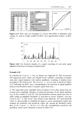
Figure 6.18. One hundred samples of a signal consisting of noise plus signal
impulses (bold lines) occurring at random times.

Example 6.10

Q: Consider the Signal & Noise dataset (see Appendix E). This set presents
100 signal plus noise values s(n) (Signal+Noise variable), consisting of random
noise plus signal impulses with random amplitude, occurring at random times
according to the Poisson law. The Signal & Noise data is shown in Figure
6.18. Determine the ROC curve corresponding to the detection of signal impulses
using several threshold values to separate signal from noise.
A: The signal plus noise amplitude shown in Figure 6.18 is often greater than the
average noise amplitude, therefore revealing the presence of the signal impulses
(e.g. at time instants 53 and 85). The discrimination between signal and noise is
made setting an amplitude threshold, Δ, such that we decide “impulse” (our rare
event) if s(n) > Δ, and “noise” (the normal event) otherwise. For each threshold
value, it’s then possible to establish the signal vs. noise classification matrix and
compute the sensitivity and specificity values. By varying the threshold (easily
done in the Signal & Noise.xls file), the corresponding sensitivity and
specificity values can be obtained, as shown in Table 6.10.