Page 264 - Applied Statistics Using SPSS, STATISTICA, MATLAB and R

6.3 Bayesian Classification 245

ˆ
Formula 6.28 allows the computation of confidence interval estimates for e ,
P
ˆ
by substituting eP in place of Pe and using the normal distribution approximation
for sufficiently large n (say, n ≥ 25). Note that formula 6.28 yields zero for the
extreme cases of Pe = 0 or Pe = 1.
In normal practice, we first compute P ˆ e by designing and evaluating the
d
classifier in the same set with n cases, eP ˆ d ( ) n . This is what we have done so far.
ˆ
As for eP , we may compute it using an independent set of n cases, eP ˆ t () n . In
t
order to have some guidance on how to choose an appropriate dimensionality ratio,
we would like to know the deviation of the expected values of these estimates from
the Bayes error. Here the expectation is computed on a population of classifiers of
the same type and trained in the same conditions. Formulas for these expectations,
Ε[ eP ˆ d () n ] and Ε[ eP ˆ t () n ], are quite intricate and can only be computed
numerically. Like formula 6.25, they depend on the Bhattacharyya distance. A
software tool, SC Size , computing these formulas for two classes with normally
distributed features and equal covariance matrices, separated by a linear
discriminant, is included with on the book CD. SC Size also allows the
computation of confidence intervals of these estimates, using formula 6.28.

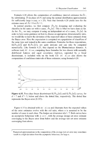
Figure 6.15. Two-class linear discriminant Ε[ eP ˆ d ( ) n ] and Ε[ eP ˆ t ( ) n ] curves, for
2
d = 7 and δ = 3, below and above the dotted line, respectively. The dotted line
represents the Bayes error (0.193).

Figure 6.15 is obtained with SC Size and illustrates how the expected values
of the error estimates evolve with the n/d ratio, where n is assumed to be the
number of cases in each class. The feature set dimension id d = 7. Both curves have
4
an asymptotic behaviour with n → ∞ , with the average design set error estimate
converging to the Bayes error from below and the average test set error estimate
converging from above.

4
Numerical approximations in the computation of the average test set error may sometimes
result in a slight deviation from the asymptotic behaviour, for large n.