Page 261 - Applied Statistics Using SPSS, STATISTICA, MATLAB and R

242 6 Statistical Classification

than for class 2 (0.218). Case #61 is also misclassified, but with a small difference
of posterior probabilities. Borderline cases as case #61 could be re-analysed, e.g.
using more features.

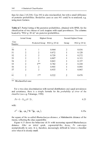
Table 6.7. Partial listing of the posterior probabilities, obtained with SPSS, for the
classification of two classes of cork stoppers with equal prevalences. The columns
headed by “P(G=g | D=d)” are posterior probabilities.

Actual Group Highest Group Second Highest Group
Case Predicted Group P(G=g | D=d) Group P(G=g | D=d)
Number
…
50 1 1 0.964 2 0.036
51 2 2 0.872 1 0.128
52 2 2 0.728 1 0.272
53 2 2 0.887 1 0.113
54 2 2 0.843 1 0.157
55 2 1** 0.782 2 0.218
56 2 2 0.905 1 0.095
57 2 2 0.935 1 0.065
…
61 2 1** 0.522 2 0.478
…
** Misclassified case

For a two-class discrimination with normal distributions and equal prevalences
and covariance, there is a simple formula for the probability of error of the
classifier (see e.g. Fukunaga, 1990):

Pe = 1 N− 1 , 0 (δ ) 2 / , 6.25

with:

2 = ( δ 1 2 )µ − ’ Σ − 1 ( µ 1 µ 2 )µ − , 6.25a

the square of the so-called Bhattacharyya distance, a Mahalanobis distance of the
means, reflecting the class separability.
Figure 6.13 shows the behaviour of Pe with increasing squared Bhattacharyya
distance. After an initial quick, exponential-like decay, Pe converges
asymptotically to zero. It is, therefore, increasingly difficult to lower a classifier
error when it is already small.