Page 269 - Applied Statistics Using SPSS, STATISTICA, MATLAB and R

250 6 Statistical Classification

There is a compromise to be made between sensitivity and specificity. This
compromise is made more patent in the ROC curve, which was obtained with
SPSS, and corresponds to eight different threshold values, as shown in Figure
6.19a (using the Data worksheet of Signal & Noise.xls ). Notice that
given the limited number of threshold values, the ROC curve has a stepwise aspect,
with different values of the FPR corresponding to the same sensitivity, as also
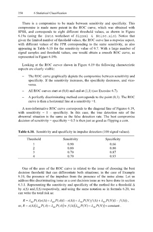
appearing in Table 6.10 for the sensitivity value of 0.7. With a large number of
signal samples and threshold values, one would obtain a smooth ROC curve, as
represented in Figure 6.19b.

Looking at the ROC curves shown in Figure 6.19 the following characteristic
aspects are clearly visible:

− The ROC curve graphically depicts the compromise between sensitivity and
specificity. If the sensitivity increases, the specificity decreases, and vice-
versa.
− All ROC curves start at (0,0) and end at (1,1) (see Exercise 6.7).
− A perfectly discriminating method corresponds to the point (0,1). The ROC
curve is then a horizontal line at a sensitivity =1.

A non-informative ROC curve corresponds to the diagonal line of Figures 6.19,
with sensitivity = 1 – specificity. In this case, the true detection rate of the
abnormal situation is the same as the false detection rate. The best compromise
decision of sensitivity = specificity = 0.5 is then just as good as flipping a coin.

Table 6.10. Sensitivity and specificity in impulse detection (100 signal values).

Threshold Sensitivity Specificity
1 0.90 0.66
2 0.80 0.80
3 0.70 0.87
4 0.70 0.93

One of the uses of the ROC curve is related to the issue of choosing the best
decision threshold that can differentiate both situations; in the case of Example
6.10, the presence of the impulses from the presence of the noise alone. Let us
address this discriminating issue as a cost decision issue as we have done in section
6.3.1. Representing the sensitivity and specificity of the method for a threshold ∆
by s(∆) and f(∆) respectively, and using the same notation as in formula 6.20, we
can write the total risk as:

R = λ aa P (A )s (∆ ) + λ an P (A )( 1− s (∆ )) + λ na P (N ) f (∆ ) + λ nn P (N )( 1− f (∆ )) ,
or, R = s (∆ ( ) λ aa P (A ) − λ an P (A ) ) + f (∆ ( ) λ na P (N ) − λ nn P (N ) ) constant+ .