Page 275 - Applied Statistics Using SPSS, STATISTICA, MATLAB and R

256 6 Statistical Classification

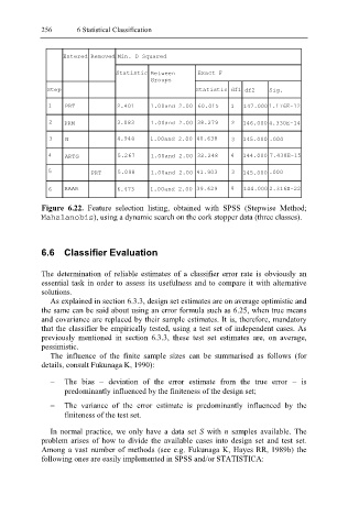
Entered Removed Min. D Squared

Statistic Between Exact F
Groups
Step Statistic df1 df2 Sig.
1 PRT 2.401 1.00and 2.00 60.015 1 147.000 1.176E-12

2 PRM 3.083 1.00and 2.00 38.279 2 146.000 4.330E-14
3 N 4.944 1.00and 2.00 40.638 3 145.000 .000

4 ARTG 5.267 1.00and 2.00 32.248 4 144.000 7.438E-15
5 PRT 5.098 1.00and 2.00 41.903 3 145.000 .000

6 RAAR 6.473 1.00and 2.00 39.629 4 144.000 2.316E-22

Figure 6.22. Feature selection listing, obtained with SPSS (Stepwise Method;
Mahalanobis ), using a dynamic search on the cork stopper data (three classes).

6.6 Classifier Evaluation

The determination of reliable estimates of a classifier error rate is obviously an
essential task in order to assess its usefulness and to compare it with alternative
solutions.
As explained in section 6.3.3, design set estimates are on average optimistic and
the same can be said about using an error formula such as 6.25, when true means
and covariance are replaced by their sample estimates. It is, therefore, mandatory
that the classifier be empirically tested, using a test set of independent cases. As
previously mentioned in section 6.3.3, these test set estimates are, on average,
pessimistic.
The influence of the finite sample sizes can be summarised as follows (for
details, consult Fukunaga K, 1990):

− The bias − deviation of the error estimate from the true error − is
predominantly influenced by the finiteness of the design set;
− The variance of the error estimate is predominantly influenced by the
finiteness of the test set.

In normal practice, we only have a data set S with n samples available. The
problem arises of how to divide the available cases into design set and test set.
Among a vast number of methods (see e.g. Fukunaga K, Hayes RR, 1989b) the
following ones are easily implemented in SPSS and/or STATISTICA: