Page 59 - Applied Statistics Using SPSS, STATISTICA, MATLAB and R

38 2 Presenting and Summarising the Data

2.1.2.4 R

Let us consider the meteo data frame created in 2.1.1.4. Every data column can be
extracted from this data frame using its name followed by the column name with
the “$” symbol in between. Thus:

> meteo$PMax

lists the values of the PMax column. We may then proceed as follows:

PClass <- 1 + (meteo$PMax>20) + (meteo$PMax>80)

creating a vector for the needed new variable. The only thing remaining to be done
is to bind this new vector to the data frame, as follows:

> meteo <- cbind(meteo,PClass)
> meteo
PMax RainDays T80 T81 T82 PClass
1 181 143 36 39 37 3
2 114 132 35 39 36 3
...

One can get rid of the clumsy $ -notation to qualify data frame variables by
using the ach att command:

> attach(meteo)

In this way variable names always respect to the attached data frame. From now
on we will always assume that an attach operation has been performed. (Whenever
needed one may undo it with detach . )
Indexing data frames is straightforward. One just needs to specify the indices
between square brackets. Some examples: meteo[2,5] and T82[2] mean the
same thing: the value of T82, 36, for the second row (case); meteo[2,] is the
whole second row; meteo[ 3:5,2] is the sub-vector containing the RainDays
values for the cases 3 through 5, i.e., 125, 111 and 102.
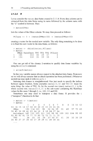
Sometimes one may need to transpose a data frame. R provides the t
(“transpose”) function to do that:

> meteo <- t(meteo)
> meteo
1 2 3 4 5 6 7 8 9 10 11 12
13 14 15 16 17 18 19 20 21 22 23 24 25
PMax 181 114 101 80 36 24 39 31 49 57 72 60
36 45 36 28 41 13 14 16 8 18 24 37 14
RainDays 143 132 125 111 102 98 96 109 102 104 95 85
92 90 83 81 79 77 75 80 72 72 71 71 70
T80 36 35 36 34 37 40 37 41 38 32 36 39
36 40 37 37 38 40 37 39 39 41 38 38 35
...