Page 61 - Applied Statistics Using SPSS, STATISTICA, MATLAB and R

40 2 Presenting and Summarising the Data

the “Commands” frames. SPSS and STATISTICA commands are described in
terms of menu options separated by “;” in the “Commands” frames. In this case
one may read “,” as “followed by”. For MATLAB and R functions “;” is simply a
separator. Alternative menu options or functions are separated by “|”.
In the following we also provide many examples illustrating the statistical
analysis procedures. We assume that the datasets used throughout the examples are
available as conveniently formatted data files ( *.sav for SPSS, *. sta for
STATISTICA, *.mat for MATLAB, files containing data frames for R).
“Example” frames end with .

2.2.1 Counts and Bar Graphs

Tables of counts and bar graphs are used to present discrete data. Denoting by X
the discrete random variable associated to the data, the table of counts – also know
as tally sheet – gives us:

– The absolute frequencies (counts), n k;
– The relative frequencies (or simply, frequencies) of occurrence f k = n k/n,

for each discrete value (category), x k, of the random variable X (n is the total
number of cases).

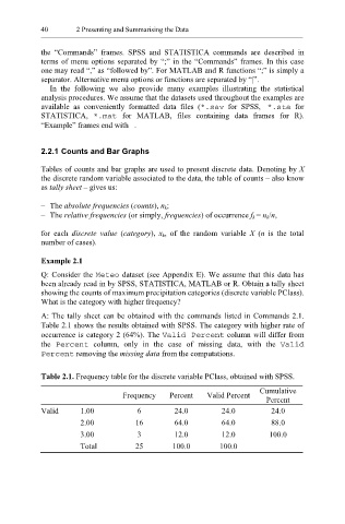
Example 2.1
Q: Consider the Meteo dataset (see Appendix E). We assume that this data has
been already read in by SPSS, STATISTICA, MATLAB or R. Obtain a tally sheet
showing the counts of maximum precipitation categories (discrete variable PClass).
What is the category with higher frequency?

A: The tally sheet can be obtained with the commands listed in Commands 2.1.
Table 2.1 shows the results obtained with SPSS. The category with higher rate of
occurrence is category 2 (64%). The Valid Percent column will differ from
the Percent column, only in the case of missing data, with the Valid
Percent removing the missing data from the computations.

Table 2.1. Frequency table for the discrete variable PClass, obtained with SPSS.
Cumulative
Frequency Percent Valid Percent
Percent
Valid 1.00 6 24.0 24.0 24.0
2.00 16 64.0 64.0 88.0
3.00 3 12.0 12.0 100.0
Total 25 100.0 100.0