Page 60 - Applied Statistics Using SPSS, STATISTICA, MATLAB and R

2.2 Presenting the Data 39

Sorting a vector can be performed with the function so rt . One often needs to
sort data frame variables according to a certain ordering of one or more of its
variables. Imagine that one wanted to get the sorted list of the maximum
precipitation variable, PMax , of the mete o data frame. The procedure to follow
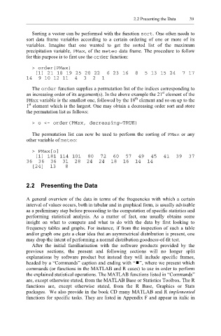
for this purpose is to first use the order function:

> order(PMax)
[1] 21 18 19 25 20 22 6 23 16 8 5 13 15 24 7 17
14 9 10 12 11 4 3 2 1

The order function supplies a permutation list of the indices corresponding to
st
an increasing order of its argument(s). In the above example the 21 element of the
th
PMax variable is the smallest one, followed by the 18 element and so on up to the
st
1 element which is the largest. One may obtain a decreasing order sort and store
the permutation list as follows:

> o <- order(PMax, decreasing=TRUE)

The permutation list can now be used to perform the sorting of PMax or any
other variable of meteo :

> PMax[o]
[1] 181 114 101 80 72 60 57 49 45 41 39 37
36 36 36 31 28 24 24 18 16 14 14
[24] 13 8

2.2 Presenting the Data

A general overview of the data in terms of the frequencies with which a certain
interval of values occurs, both in tabular and in graphical form, is usually advisable
as a preliminary step before proceeding to the computation of specific statistics and
performing statistical analysis. As a matter of fact, one usually obtains some
insight on what to compute and what to do with the data by first looking to
frequency tables and graphs. For instance, if from the inspection of such a table
and/or graph one gets a clear idea that an asymmetrical distribution is present, one
may drop the intent of performing a normal distribution goodness-of-fit test.
After the initial familiarisation with the software products provided by the
previous sections, the present and following sections will no longer split
explanations by software product but instead they will include specific frames,
”
headed by a “Commands” caption and ending with “ , where we present which
commands (or functions in the MATLAB and R cases) to use in order to perform
the explained statistical operations. The MATLAB functions listed in “Commands”
are, except otherwise stated, from the MATLAB Base or Statistics Toolbox. The R
functions are, except otherwise stated, from the R Base, Graphics or Stats
packages. We also provide in the book CD many MATLAB and R implemented
functions for specific tasks. They are listed in Appendix F and appear in italic in