Page 63 - Applied Statistics Using SPSS, STATISTICA, MATLAB and R

42 2 Presenting and Summarising the Data

With STATISTICA, the variable specification window pops up when clicking
the Variabl es tab in the Descriptive Statistics window. One can
select variables with the mouse or edit their identification numbers in a text box.
For instance, editing “2-4”, means that one wishes the analysis to be performed
starting from variable v2 up to variable v4 . There is also a Select All
variables button. The frequency table is outputted into a specific scroll-sheet that is
part of a session workbook file, which constitutes a session logbook that can be
saved ( *.stw file) and opened at a later session. The entire scroll-sheet (or any
part of the screen) can be copied to the clipboard (from where it can be pasted into
a document in the normal way), using the Screen Catcher tool of the Edit
menu. As an alternative, one can also copy the contents of the table alone in the
normal way.
The MATLAB tabulate function computes a 3-column matrix, such that the
first column contains the different values of the argument, the second column
values are absolute frequencies (counts), and the third column are these frequencies
in percentage. For the PClass example we have:

» t=tabulate(PClass)
t =
1 6 24
2 16 64
3 3 12

Text output of MATLAB can be copied and pasted in the usual way.
The R table function – ta ble(PClass) for the example – computes the
counts. The function prop. table(x) computes proportions of each vector x
element. In order to obtain the information of the above last column one should use
prop.table(table(PClass)) . Text output of the R console can be copied
and pasted in the usual way.

70

60
50
40
30
20
Percent 10 0

1.00 2.00 3.00
PCLASS
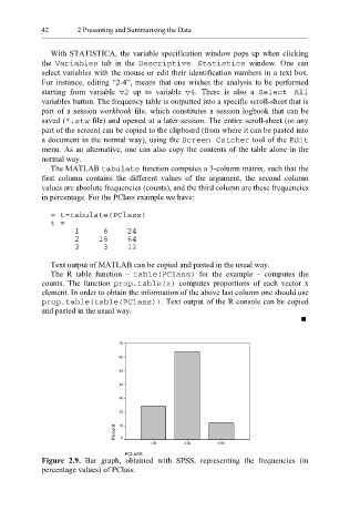
Figure 2.9. Bar graph, obtained with SPSS, representing the frequencies (in
percentage values) of PClass.