Page 86 - Artificial Intelligence for Computational Modeling of the Heart

56 Chapter 2 Implementation of a patient-specific cardiac model

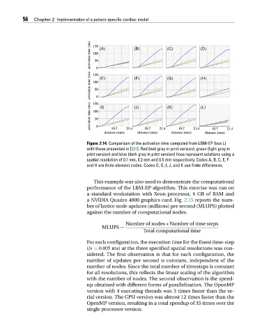
Figure 2.14. Comparison of the activation time computed from LBM-EP (box L)
with those presented in [221]. Red (mid gray in print version), green (light gray in
print version) and blue (dark gray in print version) lines represent solutions using a
spatial resolution of 0.1 mm, 0.2 mm and 0.5 mm respectively. Codes A, B, C, E, F
and H are finite element codes. Codes D, G, I, J, and K use finite differences.

This example was also used to demonstrate the computational
performance of the LBM-EP algorithm. This exercise was run on
a standard workstation with Xeon processor, 6 GB of RAM and
a NVIDIA Quadro 4000 graphics card. Fig. 2.15 reports the num-
ber of lattice node updates (millions) per second (MLUPS) plotted
against the number of computational nodes.

Number of nodes ∗ Number of time steps
MLUPS =
Total computational time

For each configuration, the execution time for the finest time-step
(δt = 0.005 ms) at the three specified spatial resolutions was con-
sidered. The first observation is that for each configuration, the
number of updates per second is constant, independent of the
number of nodes. Since the total number of timesteps is constant
for all resolutions, this reflects the linear scaling of the algorithm
with the number of nodes. The second observation is the speed-
up obtained with different forms of parallelization. The OpenMP
version with 4 executing threads was 3 times faster than the se-
rial version. The GPU version was almost 12 times faster than the
OpenMP version, resulting in a total speedup of 35 times over the
single processor version.