Page 83 - Artificial Intelligence for Computational Modeling of the Heart

Chapter 2 Implementation of a patient-specific cardiac model 53

functions f ={f 1 ,f 2 ,...,f N },where f i (x,t) = f(x,e i ,t),and each
component is strictly a function of only space and time. The ve-
locity vectors e i are chosen to be the links connecting every lattice
node to its 6 nearest neighbors on the Cartesian grid, as well as a
link to itself. The trans-membrane potential is related to the distri-

bution function through v = f i . The dynamics of the distribu-
i
tion function evolves through the following linearized Boltzmann
equation:
∂f i (0)
+ e i ·∇f i = Ω ij (f j − f ) + s i , (2.1)
∂t j
where Ω ij is a matrix which operates on the deviation of the dis-
(0)
tribution function from its equilibrium value f = v/7 and s i is
i
the contribution of any sources (ionic and stimulus currents). The
analysis is significantly easier operating in a space of moments of
the distribution function, instead of directly operating over f.For
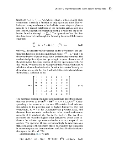
this reason, we introduce an orthogonal transformation matrix M
which transforms the distribution function into a set of linearly in-
dependent moments. For the 7-velocity lattice introduced above,
the matrix M is chosen to be:
⎡ ⎤
1 1 1 1 1 1 1
⎢ 1 −1 0 0 0 0 0 ⎥
⎢ ⎥
⎢ 0 0 1 −1 0 0 0 ⎥
⎢ ⎥
M = ⎢ 0 0 0 0 1 −1 0 ⎥ . (2.2)
⎢ ⎥
⎢ 1 1 1 1 1 1 −6 ⎥
⎢ ⎥
⎣ 1 1 −1 −1 0 0 0 ⎦
1 1 1 1 −2 −2 0
The moments corresponding to the equilibrium distribution func-
T
tion can be seen to be m (0) = Mf (0) = [v,0,0,0,0,0,0] .Corre-
spondingly, the moment vector m = Mf contains local informa-
tion related to the potential and its higher derivatives. The first
component, m 0 = v is the transmembrane potential itself, and
the next three moments can be shown to be related to the com-
ponents of its gradient, (∂v/∂x 1 ,∂v/∂x 2 ,∂v/∂x 3 ). The last three
moments are related to higher order derivatives, which don’t in-
fluence the solution up to second order accuracy in spatial res-
olution. The operator, Ω can correspondingly be rewritten as a
transformation to the moment space, followed by the relaxation
in moment space and then transform back into distribution func-
tion space, i.e., Ω = M −1 SM.
Discretizing Eq. (2.1), we get:
f(x + ce i δt,t + δt) = f(x,t) − M −1 SM(f − f (0) ) + δts(x,t), (2.3)