Page 85 - Artificial Intelligence for Computational Modeling of the Heart

Chapter 2 Implementation of a patient-specific cardiac model 55

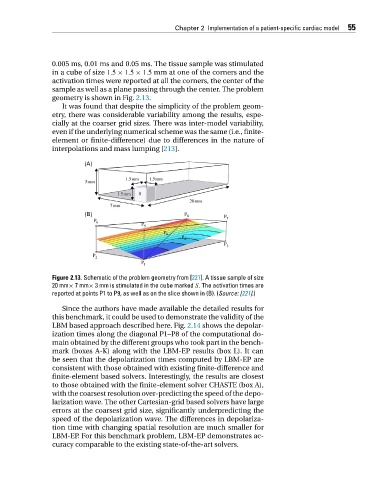
0.005 ms, 0.01 ms and 0.05 ms. The tissue sample was stimulated
in a cube of size 1.5 × 1.5 × 1.5 mm at one of the corners and the
activation times were reported at all the corners, the center of the
sample as well as a plane passing through the center. The problem
geometry is shown in Fig. 2.13.
It was found that despite the simplicity of the problem geom-
etry, there was considerable variability among the results, espe-
cially at the coarser grid sizes. There was inter-model variability,
even if the underlying numerical scheme was the same (i.e., finite-
element or finite-difference) due to differences in the nature of
interpolations and mass lumping [213].

Figure 2.13. Schematic of the problem geometry from [221]. A tissue sample of size
20 mm× 7mm× 3 mm is stimulated in the cube marked S. The activation times are
reported at points P1 to P9, as well as on the slice shown in (B). (Source: [221].)

Since the authors have made available the detailed results for
this benchmark, it could be used to demonstrate the validity of the
LBM based approach described here. Fig. 2.14 shows the depolar-
ization times along the diagonal P1–P8 of the computational do-
main obtained by the different groups who took part in the bench-
mark (boxes A-K) along with the LBM-EP results (box L). It can
be seen that the depolarization times computed by LBM-EP are
consistent with those obtained with existing finite-difference and
finite-element based solvers. Interestingly, the results are closest
to those obtained with the finite-element solver CHASTE (box A),
with the coarsest resolution over-predicting the speed of the depo-
larization wave. The other Cartesian-grid based solvers have large
errors at the coarsest grid size, significantly underpredicting the
speed of the depolarization wave. The differences in depolariza-
tion time with changing spatial resolution are much smaller for
LBM-EP. For this benchmark problem, LBM-EP demonstrates ac-
curacy comparable to the existing state-of-the-art solvers.