Page 742 - Automotive Engineering Powertrain Chassis System and Vehicle Body

Exterior noise: Assessment and control C HAPTER 22.1

(valve). However, equation (22.1.47) will tend to predict but not on the other, producing a sudden drop in dis-
much higher flow rates than are encountered with prac- charge coefficient that subsequently recovers with fur-
tical engines, due to the large number of simplifying as- ther valve lift. At high valve lifts, the flow is detached
sumptions that went into its derivation. One way to from both sides, and the so-called free-jet is formed.
correct this effect is to introduce a discharge coefficient The discharge coefficients for outflow through the
c d where inlet valve (reverse flow) are generally higher (around 0.7
up to L v /D ¼ 0.2, then falling to 0.5 at L v /D ¼ 0.4).
A e Flow loss coefficients (rather than discharge co-
c ¼ (22.1.48)
d
A r efficients) are commonly used in commercial engine
simulations (AVL, 2000). These are defined as the ratio
and A e is the effective area and A r is some suitable ref- between the actual mass flow and the loss-free isentropic
erence area. The effective area (Annand and Roe, 1974) mass flow for the same stagnation pressure and the same
is the outlet area of an imaginary frictionless nozzle which pressure ratio (AVL, 2000). The difference between
would pass the required flow when drawing from a large a discharge coefficient and a flow loss coefficient is
constant pressure reservoir and discharging into another important. The discharge coefficient applies to flow be-
reservoir. The reference area can be the cross-sectional tween stagnant reservoirs passing through a frictionless
area of any suitable part of the real flow path such as the nozzle. The flow loss coefficient applies to steady or
curtain area under the open valve. pulsating flow through the cylinder head.
Measured discharge coefficients can be used to cal- Flow loss coefficients (such as those shown in Figs.
culate the effective area for a given reference area, and 22.1-8 and 22-1-9) are often measured using steady flow
hence equation (22.1.47) becomes: on a bench (Blair and Drouin, 1996). Sometimes, they
1=2 are measured using pulsed flow (for instance, Fukutani
p 01 A e 2g 2 p 2 2=g p 2 g 1=g and Watanabe (1982)) in order to improve the realism of
_ m ¼ 1
a 01 g 1 p 01 p 01 the model represented by equation (22.1.49).
(22.1.49) An example for an intake port is given in Fig. 22.1-8
and an example for an exhaust port in Fig. 22.1-9.
The most well-known discharge coefficients for inflow For the flow loss coefficients shown in Figs. 22.1-8 and
through the intake valve are given in Annand and Roe 22.1-9
(1974) for a reference area equal to the curtain area
2
under the open valve d p
vi
A e ¼ coefficient (22.1.51)
4
A r ¼ pDL v (22.1.50)
where d vi is the inner valve seat diameter (reference di-
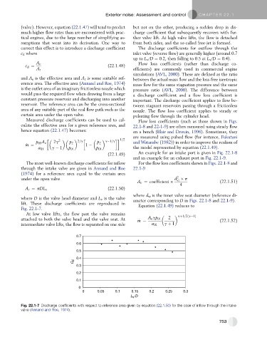
where D is the valve head diameter and L v is the valve ameter corresponding to D in Figs. 22.1-8 and 22.1-9).
lift. These discharge coefficients are reproduced in Equation (22.1.49) reduces to
Fig. 22.1-7.
At low valve lifts, the flow past the valve remains gþ1=2ðg 1Þ
attached to both the valve head and the valve seat. At _ m ¼ A e gp 01 2 (22.1.52)
intermediate valve lifts, the flow is separated on one side a 01 g þ 1

0.7
0.6
0.5
0.4
C d
0.3
0.2
0.1
0
0 0.05 0.1 0.15 0.2 0.25 0.3
L v /D

Fig. 22.1-7 Discharge coefficients with respect to reference area given by equation (22.1.50) for the case of inflow through the intake
valve (Annand and Roe, 1974).

753