Page 101 - Autonomous Mobile Robots

84 Autonomous Mobile Robots

0°
scan start
200

50
150
100 40

50 Concrete step 30
Range (m) 0 Trees 20

–50 Nonmetallic pole
10
Fence
–100 Fence
0
Range bin at
–150 231°
–10
–200
–200 –150 –100 –50 0 50 100 150 200
Range (m)

◦
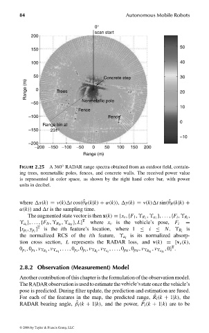
FIGURE 2.25 A 360 RADAR range spectra obtained from an outdoor field, contain-
ing trees, nonmetallic poles, fences, and concrete walls. The received power value
is represented in color space, as shown by the right hand color bar, with power
units in decibel.

where x(k) = v(k) t cos( ˆ θ R (k|k) + α(k)), y(k) = v(k) t sin( ˆ θ R (k|k) +
α(k)) and t is the sampling time.
,
The augmented state vector is then x(k) =[x v , {F 1 , ϒ R 1 , ϒ a 1 }, ... , {F i , ϒ R i
T
}, L] =
ϒ a i }, ... , {F N , ϒ R N , ϒ a N where x v is the vehicle’s pose, F i
T
] is
[x p i , y p i is the ith feature’s location, where 1 ≤ i ≤ N. ϒ R i
is its normalized absorp-
the normalized RCS of the ith feature, ϒ a i
tion cross section, L represents the RADAR loss, and v(k) =[v v (k),
T
,0] .
0 p 1 ,0 p 1 , v ϒ R 1 , v ϒ a 1 , ... ,0 p i ,0 p i , v ϒ R i , v ϒ a i , ... ,0 p N ,0 p N , v ϒ R N , v ϒ a N
2.8.2 Observation (Measurement) Model
Another contribution of this chapter is the formulation of the observation model.
The RADAR observation isused to estimate the vehicle’sstate once the vehicle’s
pose is predicted. During filter update, the prediction and estimation are fused.
For each of the features in the map, the predicted range, R i (k + 1|k), the
ˆ
RADAR bearing angle, ˆ β i (k + 1|k), and the power, P i (k + 1|k) are to be
ˆ

© 2006 by Taylor & Francis Group, LLC

FRANKL: “dk6033_c002” — 2006/3/31 — 17:29 — page 84 — #44